You can run this notebook in a live session or view it on Github.

Calculate skill of a MJO Index of SubX model GEOS_V2p1 as function of daily lead time

In this example, we demonstrate:

1. How to remotely access data from the Subseasonal Experiment (SubX) hindcast database and set it up to be used in climpred.

2. How to calculate the Anomaly Correlation Coefficient (ACC) using daily data with climpred

3. How to calculate and plot historical forecast skill of the real-time multivariate MJO (RMM) indices as function of lead time.

The Subseasonal Experiment (SubX)

Further information on SubX is available from Pegion et al. [2019] and the SubX project website.

The SubX public database is hosted on the International Research Institute for Climate and Society (IRI) data server http://iridl.ldeo.columbia.edu/SOURCES/.Models/.SubX/.

Since the SubX data server is accessed via this notebook, the time for the notebook to run may is several minutes and will vary depending on the speed that data can be downloaded. This is a large dataset, so please be patient. If you prefer to download SubX data locally, scripts are available from https://github.com/kpegion/SubX.

Definitions

RMM

Two indices (RMM1 and RMM2) are used to represent the MJO. Together they define the MJO based on 8 phases and can represent both the phase and amplitude of the MJO [Wheeler and Hendon, 2004]. This example uses the observed RMM1 provided by Matthew Wheeler at the Center for Australian Weather and Climate Research. It is the version of the indices in which interannual variability has not been removed.

Skill of RMM

Traditionally, the skill of the RMM is calculated as a bivariate correlation encompassing the skill of the two indices together [Gottschalck et al., 2010, Rashid et al., 2011]. Currently, climpred does not have the functionality to calculate the bivariate correlation, thus the anomaly correlation coefficient for RMM1 index is calculated here as a demonstration. The bivariate correlation metric will be added in a future version of climpred.

# linting
%load_ext nb_black
%load_ext lab_black

---------------------------------------------------------------------------
ModuleNotFoundError                       Traceback (most recent call last)
Cell In[1], line 2
      1 # linting
----> 2 get_ipython().run_line_magic('load_ext', 'nb_black')
      3 get_ipython().run_line_magic('load_ext', 'lab_black')

File ~/checkouts/readthedocs.org/user_builds/climpred/conda/latest/lib/python3.9/site-packages/IPython/core/interactiveshell.py:2456, in InteractiveShell.run_line_magic(self, magic_name, line, _stack_depth)
   2454     kwargs['local_ns'] = self.get_local_scope(stack_depth)
   2455 with self.builtin_trap:
-> 2456     result = fn(*args, **kwargs)
   2458 # The code below prevents the output from being displayed
   2459 # when using magics with decorator @output_can_be_silenced
   2460 # when the last Python token in the expression is a ';'.
   2461 if getattr(fn, magic.MAGIC_OUTPUT_CAN_BE_SILENCED, False):

File ~/checkouts/readthedocs.org/user_builds/climpred/conda/latest/lib/python3.9/site-packages/IPython/core/magics/extension.py:33, in ExtensionMagics.load_ext(self, module_str)
     31 if not module_str:
     32     raise UsageError('Missing module name.')
---> 33 res = self.shell.extension_manager.load_extension(module_str)
     35 if res == 'already loaded':
     36     print("The %s extension is already loaded. To reload it, use:" % module_str)

File ~/checkouts/readthedocs.org/user_builds/climpred/conda/latest/lib/python3.9/site-packages/IPython/core/extensions.py:76, in ExtensionManager.load_extension(self, module_str)
     69 """Load an IPython extension by its module name.
     70 
     71 Returns the string "already loaded" if the extension is already loaded,
     72 "no load function" if the module doesn't have a load_ipython_extension
     73 function, or None if it succeeded.
     74 """
     75 try:
---> 76     return self._load_extension(module_str)
     77 except ModuleNotFoundError:
     78     if module_str in BUILTINS_EXTS:

File ~/checkouts/readthedocs.org/user_builds/climpred/conda/latest/lib/python3.9/site-packages/IPython/core/extensions.py:91, in ExtensionManager._load_extension(self, module_str)
     89 with self.shell.builtin_trap:
     90     if module_str not in sys.modules:
---> 91         mod = import_module(module_str)
     92     mod = sys.modules[module_str]
     93     if self._call_load_ipython_extension(mod):

File ~/checkouts/readthedocs.org/user_builds/climpred/conda/latest/lib/python3.9/importlib/__init__.py:127, in import_module(name, package)
    125             break
    126         level += 1
--> 127 return _bootstrap._gcd_import(name[level:], package, level)

File <frozen importlib._bootstrap>:1030, in _gcd_import(name, package, level)

File <frozen importlib._bootstrap>:1007, in _find_and_load(name, import_)

File <frozen importlib._bootstrap>:984, in _find_and_load_unlocked(name, import_)

ModuleNotFoundError: No module named 'nb_black'

import warnings

import matplotlib.pyplot as plt

import xarray as xr
import pandas as pd
import numpy as np

from climpred import HindcastEnsemble
import climpred

warnings.filterwarnings("ignore")

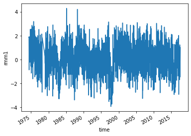
Read the observed RMM Indices.

obsds = climpred.tutorial.load_dataset("RMM-INTERANN-OBS")[["rmm1"]].dropna(
    "time"
)  # Get rid of missing times.

obsds["rmm1"].plot()

[<matplotlib.lines.Line2D at 0x14d9e5b20>]

Read the SubX RMM1 data for the GMAO-GEOS_V2p1 model from the SubX data server. It is important to note that the SubX data contains weekly initialized forecasts where the init day varies by model. SubX data may have all NaNs for initial dates in which a model does not make a forecast, thus we apply dropna over the S=init dimension when how=all data for a given S=init is missing. This can be slow, but allows the rest of the calculations to go more quickly.

Note that we ran the dropna operation offline and then uploaded the post-processed SubX dataset to the climpred-data repo for the purposes of this demo. This is how you can do this manually:

url = 'http://iridl.ldeo.columbia.edu/SOURCES/.Models/.SubX/.GMAO/.GEOS_V2p1/.hindcast/.RMM/.RMM1/dods/'
fcstds = xr.open_dataset(url, decode_times=False, chunks={'S': 1, 'L': 45}).dropna(dim='S',how='all')

fcstds = climpred.tutorial.load_dataset("GMAO-GEOS-RMM1", decode_times=False)
fcstds

<xarray.Dataset>
Dimensions:  (S: 510, M: 4, L: 45)
Coordinates:
  * S        (S) float32 1.424e+04 1.425e+04 1.426e+04 ... 2.044e+04 2.045e+04
  * M        (M) float32 1.0 2.0 3.0 4.0
  * L        (L) float32 0.5 1.5 2.5 3.5 4.5 5.5 ... 40.5 41.5 42.5 43.5 44.5
Data variables:
    RMM1     (S, M, L) float32 -0.03237 0.1051 0.1946 ... -0.1499 0.08326 0.1389
Attributes:
    Conventions:  IRIDL

xarray.Dataset

• Dimensions:
  • S: 510
  • M: 4
  • L: 45
• Coordinates: (3)
  • S
    (S)
    float32
    1.424e+04 1.425e+04 ... 2.045e+04

    long_name :

    Start Time

    calendar :

    standard

    standard_name :

    forecast_reference_time

    pointwidth :

    0.0

    gridtype :

    0

    units :

    days since 1960-01-01

    array([14245., 14250., 14255., ..., 20439., 20444., 20449.], dtype=float32)

  • M
    (M)
    float32
    1.0 2.0 3.0 4.0

    long_name :

    Ensemble Member

    standard_name :

    realization

    pointwidth :

    1.0

    gridtype :

    0

    units :

    ids

    array([1., 2., 3., 4.], dtype=float32)

  • L
    (L)
    float32
    0.5 1.5 2.5 3.5 ... 42.5 43.5 44.5

    long_name :

    Lead

    standard_name :

    forecast_period

    pointwidth :

    1.0

    gridtype :

    0

    units :

    days

    array([ 0.5,  1.5,  2.5,  3.5,  4.5,  5.5,  6.5,  7.5,  8.5,  9.5, 10.5, 11.5,
           12.5, 13.5, 14.5, 15.5, 16.5, 17.5, 18.5, 19.5, 20.5, 21.5, 22.5, 23.5,
           24.5, 25.5, 26.5, 27.5, 28.5, 29.5, 30.5, 31.5, 32.5, 33.5, 34.5, 35.5,
           36.5, 37.5, 38.5, 39.5, 40.5, 41.5, 42.5, 43.5, 44.5], dtype=float32)

• Data variables: (1)
  • RMM1
    (S, M, L)
    float32
    ...

    pointwidth :

    0.0

    long_name :

    RMM1

    units :

    unitless

    array([[[-0.032366,  0.105126, ...,  1.778099,  1.803143],
            [ 0.006499,  0.158598, ...,  0.826527,  0.743905],
            [ 0.014169,  0.147751, ...,  1.170505,  1.230083],
            [-0.014136,  0.142899, ...,  1.239202,  1.26709 ]],
    
           [[ 0.222802,  0.70556 , ...,  2.06537 ,  1.935836],
            [ 0.192239,  0.610177, ...,  1.658914,  1.51989 ],
            [ 0.200765,  0.662475, ...,  1.159152,  1.093163],
            [ 0.203409,  0.631355, ..., -0.66206 , -0.785497]],
    
           ...,
    
           [[ 0.167977,  0.093171, ...,  0.455726,  0.463756],
            [ 0.300361,  0.193978, ..., -0.853684, -0.762082],
            [ 0.223478,  0.095381, ..., -0.784702, -0.75755 ],
            [ 0.228956,  0.144475, ..., -0.866805, -0.977645]],
    
           [[-0.648854, -1.236488, ...,  0.467468,  0.470097],
            [-0.566065, -1.12568 , ...,  0.261335,  0.253228],
            [-0.638935, -1.209603, ..., -0.003442, -0.231822],
            [-0.603829, -1.186343, ...,  0.083258,  0.138907]]], dtype=float32)

• Attributes: (1)

  Conventions :

  IRIDL

The SubX data dimensions correspond to the following climpred dimension definitions: X=lon,L=lead,Y=lat,M=member, S=init. We will rename the dimensions to their climpred names.

fcstds = fcstds.rename({"S": "init", "L": "lead", "M": "member", "RMM1": "rmm1"})

Let’s make sure that the lead dimension is set properly for climpred. SubX data stores leads as 0.5, 1.5, 2.5, etc, which correspond to 0, 1, 2, … days since initialization. We will change the lead to be integers starting with zero.

fcstds["lead"] = (fcstds["lead"] - 0.5).astype("int")

Now we need to make sure that the init dimension is set properly for climpred. We use the xarray convenience function decode_cf to convert the numeric time into datetimes. It recognizes that this is on a 360 day calendar.

fcstds = xr.decode_cf(fcstds, decode_times=True)

climpred also requires that lead dimension has an attribute called units indicating what time units the lead is assocated with. Options are: years, seasons, months, weeks, pentads, days, hours, minutes, or seconds. For the SubX data, the lead units are days.

fcstds["lead"].attrs = {"units": "days"}

Create the HindcastEnsemble object and HindcastEnsemble.add_observations().

hindcast = HindcastEnsemble(fcstds).add_observations(obsds)
hindcast

Calculate the Anomaly Correlation Coefficient (ACC) climpred.metrics._pearson_r()

skill = hindcast.verify(
    metric="acc", comparison="e2o", dim="init", alignment="maximize"
)
skill

<xarray.Dataset>
Dimensions:  (lead: 45)
Coordinates:
  * lead     (lead) int64 0 1 2 3 4 5 6 7 8 9 ... 35 36 37 38 39 40 41 42 43 44
    skill    <U11 'initialized'
Data variables:
    rmm1     (lead) float64 0.9782 0.9719 0.9632 0.9508 ... 0.304 0.2801 0.2616
Attributes:
    Conventions:                   IRIDL
    prediction_skill_software:     climpred https://climpred.readthedocs.io/
    skill_calculated_by_function:  HindcastEnsemble.verify()
    number_of_initializations:     510
    number_of_members:             4
    alignment:                     maximize
    metric:                        pearson_r
    comparison:                    e2o
    dim:                           init
    reference:                     []

xarray.Dataset

• Dimensions:
  • lead: 45
• Coordinates: (2)
  • lead
    (lead)
    int64
    0 1 2 3 4 5 6 ... 39 40 41 42 43 44

    units :

    days

    standard_name :

    forecast_period

    long_name :

    Lead

    description :

    Forecast period is the time interval between the forecast reference time and the validity time. A period is an interval of time, or the time-period of an oscillation.

    array([ 0,  1,  2,  3,  4,  5,  6,  7,  8,  9, 10, 11, 12, 13, 14, 15, 16, 17,
           18, 19, 20, 21, 22, 23, 24, 25, 26, 27, 28, 29, 30, 31, 32, 33, 34, 35,
           36, 37, 38, 39, 40, 41, 42, 43, 44])

  • skill
    ()
    <U11
    'initialized'

    description :

    new dimension prediction skill of initialized and reference forecasts created by .verify() or .bootstrap()

    documentation :

    https://climpred.readthedocs.io/en/v2.1.7.dev40+ga522c2d.d20211213/reference_forecast.html

    array('initialized', dtype='<U11')

• Data variables: (1)
  • rmm1
    (lead)
    float64
    0.9782 0.9719 ... 0.2801 0.2616

    pointwidth :

    0.0

    long_name :

    RMM1

    units :

    None

    array([0.97824896, 0.97189502, 0.96318644, 0.95076842, 0.94041475,
           0.92822477, 0.9151771 , 0.9016461 , 0.88447295, 0.86887304,
           0.85702033, 0.8390022 , 0.82610532, 0.81098753, 0.79177509,
           0.76371731, 0.73140071, 0.71192524, 0.69532361, 0.67409687,
           0.64613392, 0.62045798, 0.60304052, 0.57694587, 0.54281267,
           0.51273148, 0.48632694, 0.47907456, 0.46396743, 0.4500141 ,
           0.43143553, 0.42453133, 0.42558115, 0.40486766, 0.3930706 ,
           0.36930495, 0.34949077, 0.35310383, 0.34532601, 0.34517177,
           0.32895868, 0.31148626, 0.30401626, 0.28014658, 0.26156093])

• Attributes: (10)

  Conventions :

  IRIDL

  prediction_skill_software :

  climpred https://climpred.readthedocs.io/

  skill_calculated_by_function :

  HindcastEnsemble.verify()

  number_of_initializations :

  510

  number_of_members :

  4

  alignment :

  maximize

  metric :

  pearson_r

  comparison :

  e2o

  dim :

  init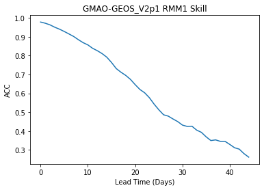

  reference :

  []

Plot the skill as a function of lead time

skill["rmm1"].plot()
plt.title("GMAO-GEOS_V2p1 RMM1 Skill")
plt.xlabel("Lead Time (Days)")
plt.ylabel("ACC")

Text(0, 0.5, 'ACC')

References

[1]

J. Gottschalck, M. Wheeler, K. Weickmann, F. Vitart, N. Savage, H. Lin, H. Hendon, D. Waliser, K. Sperber, M. Nakagawa, C. Prestrelo, M. Flatau, and W. Higgins. A Framework for Assessing Operational Madden–Julian Oscillation Forecasts: A CLIVAR MJO Working Group Project. Bulletin of the American Meteorological Society, 91(9):1247–1258, September 2010. doi:10/fcftn7.

[2]

Kathy Pegion, Ben P. Kirtman, Emily Becker, Dan C. Collins, Emerson LaJoie, Robert Burgman, Ray Bell, Timothy DelSole, Dughong Min, Yuejian Zhu, Wei Li, Eric Sinsky, Hong Guan, Jon Gottschalck, E. Joseph Metzger, Neil P Barton, Deepthi Achuthavarier, Jelena Marshak, Randal D. Koster, Hai Lin, Normand Gagnon, Michael Bell, Michael K. Tippett, Andrew W. Robertson, Shan Sun, Stanley G. Benjamin, Benjamin W. Green, Rainer Bleck, and Hyemi Kim. The Subseasonal Experiment (SubX): A Multimodel Subseasonal Prediction Experiment. Bulletin of the American Meteorological Society, 100(10):2043–2060, July 2019. doi:10/ggkt9s.

[3]

Harun A. Rashid, Harry H. Hendon, Matthew C. Wheeler, and Oscar Alves. Prediction of the Madden–Julian oscillation with the POAMA dynamical prediction system. Climate Dynamics, 36(3):649–661, February 2011. doi:10/b992k4.

[4]

Matthew C. Wheeler and Harry H. Hendon. An All-Season Real-Time Multivariate MJO Index: Development of an Index for Monitoring and Prediction. Monthly Weather Review, 132(8):1917–1932, August 2004. doi:10/d489vd.