You can run this notebook in a live session or view it on Github.

Hindcast Predictions of Equatorial Pacific SSTs

In this example, we evaluate hindcasts (retrospective forecasts) with HindcastEnsemble of sea surface temperatures in the eastern equatorial Pacific from CESM-DPLE. These hindcasts are evaluated against a forced ocean-sea ice simulation that initializes the model.

See the quick start for an analysis of time series (rather than maps) from HindcastEnsemble.

# linting
%load_ext nb_black
%load_ext lab_black

%matplotlib inline
import matplotlib.pyplot as plt
import numpy as np

import climpred
from climpred import HindcastEnsemble
import xarray as xr

xr.set_options(display_style="text")

# silence warnings if annoying
# import warnings
# warnings.filterwarnings("ignore")

<xarray.core.options.set_options at 0x10d603d30>

We’ll load in a small region of the eastern equatorial Pacific for this analysis example.

initialized = climpred.tutorial.load_dataset("CESM-DP-SST-3D")["SST"]
recon = climpred.tutorial.load_dataset("FOSI-SST-3D")["SST"]
initialized

<xarray.DataArray 'SST' (init: 64, lead: 10, nlat: 37, nlon: 26)>
[615680 values with dtype=float32]
Coordinates:
    TLAT     (nlat, nlon) float64 ...
    TLONG    (nlat, nlon) float64 ...
  * init     (init) float32 1.954e+03 1.955e+03 ... 2.016e+03 2.017e+03
  * lead     (lead) int32 1 2 3 4 5 6 7 8 9 10
    TAREA    (nlat, nlon) float64 ...
Dimensions without coordinates: nlat, nlon

These two example products cover a small portion of the eastern equatorial Pacific.

It is generally advisable to do all bias correction before instantiating a HindcastEnsemble. However, HindcastEnsemble can also be modified with HindcastEnsemble.remove_bias().

climpred requires that lead dimension has an attribute called units indicating what time units the lead is assocated with. Options are: years, seasons, months, weeks, pentads, days, hours, minutes, seconds. For the this data, the lead units are years.

initialized["lead"].attrs["units"] = "years"

hindcast = HindcastEnsemble(initialized).add_observations(recon)
hindcast

/Users/aaron.spring/Coding/climpred/climpred/utils.py:191: UserWarning: Assuming annual resolution starting Jan 1st due to numeric inits. Please change ``init`` to a datetime if it is another resolution. We recommend using xr.CFTimeIndex as ``init``, see https://climpred.readthedocs.io/en/stable/setting-up-data.html.
  warnings.warn(
/Users/aaron.spring/Coding/climpred/climpred/utils.py:191: UserWarning: Assuming annual resolution starting Jan 1st due to numeric inits. Please change ``init`` to a datetime if it is another resolution. We recommend using xr.CFTimeIndex as ``init``, see https://climpred.readthedocs.io/en/stable/setting-up-data.html.
  warnings.warn(

<climpred.HindcastEnsemble>
Initialized Ensemble:
    SST      (init, lead, nlat, nlon) float32 -0.3323 -0.3238 ... 1.179 1.123
Observations:
    SST      (time, nlat, nlon) float32 25.53 25.43 25.35 ... 27.03 27.1 27.05
Uninitialized:
    None

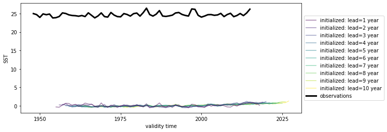
# Quick look at the HindEnsemble timeseries: only works for 1-dimensional data, therefore take spatial mean
hindcast.mean(["nlat", "nlon"]).plot()

<AxesSubplot:xlabel='validity time', ylabel='SST'>

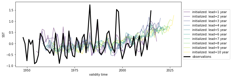
We first need to remove the same climatology that was used to drift-correct the CESM-DPLE.

recon = recon - recon.sel(time=slice(1964, 2014)).mean("time")
hindcast = hindcast.add_observations(recon)
hindcast.mean(["nlat", "nlon"]).plot()

/Users/aaron.spring/Coding/climpred/climpred/utils.py:191: UserWarning: Assuming annual resolution starting Jan 1st due to numeric inits. Please change ``init`` to a datetime if it is another resolution. We recommend using xr.CFTimeIndex as ``init``, see https://climpred.readthedocs.io/en/stable/setting-up-data.html.
  warnings.warn(

<AxesSubplot:xlabel='validity time', ylabel='SST'>

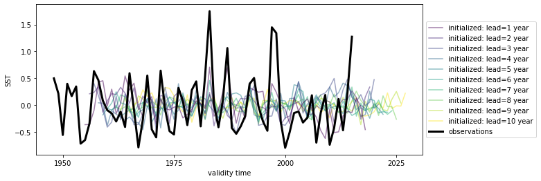
We’ll also detrend climpred.stats.rm_trend() the reconstruction over its time dimension and initialized forecast ensemble over lead.

from climpred.stats import rm_trend

hindcast_detrend = hindcast.map(rm_trend, dim="lead_or_time")

hindcast_detrend.mean(["nlat", "nlon"]).plot()

<AxesSubplot:xlabel='validity time', ylabel='SST'>

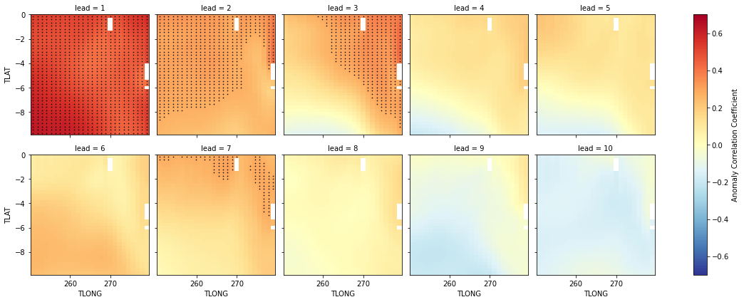
Anomaly Correlation Coefficient of SSTs

We can now compute the ACC climpred.metrics._pearson_r() over all leads and all grid cells with HindcastEnsemble.verify.

predictability = hindcast_detrend.verify(
    metric="acc", comparison="e2o", dim="init", alignment="same_verif"
)
predictability

<xarray.Dataset>
Dimensions:  (lead: 10, nlat: 37, nlon: 26)
Coordinates:
  * nlat     (nlat) int64 0 1 2 3 4 5 6 7 8 9 ... 27 28 29 30 31 32 33 34 35 36
  * nlon     (nlon) int64 0 1 2 3 4 5 6 7 8 9 ... 16 17 18 19 20 21 22 23 24 25
    TLONG    (nlat, nlon) float64 250.8 251.9 253.1 254.2 ... 276.7 277.8 278.9
  * lead     (lead) int32 1 2 3 4 5 6 7 8 9 10
    TAREA    (nlat, nlon) float64 3.661e+13 3.661e+13 ... 3.714e+13 3.714e+13
    TLAT     (nlat, nlon) float64 -9.75 -9.75 -9.75 ... -0.1336 -0.1336 -0.1336
    skill    <U11 'initialized'
Data variables:
    SST      (lead, nlat, nlon) float64 0.6272 0.6248 ... -0.05417 -0.05513
Attributes:
    prediction_skill_software:     climpred https://climpred.readthedocs.io/
    skill_calculated_by_function:  HindcastEnsemble.verify()
    number_of_initializations:     64
    alignment:                     same_verif
    metric:                        pearson_r
    comparison:                    e2o
    dim:                           init
    reference:                     []

We use the pval keyword to get associated p-values for our ACCs. We can then mask our final maps based on .

significance = hindcast_detrend.verify(
    metric="p_pval", comparison="e2o", dim="init", alignment="same_verif"
)

# Mask latitude and longitude by significance for stippling.
siglat = significance.TLAT.where(significance.SST <= 0.05)
siglon = significance.TLONG.where(significance.SST <= 0.05)

p = predictability.SST.plot.pcolormesh(
    x="TLONG",
    y="TLAT",
    col="lead",
    col_wrap=5,
    cbar_kwargs={"label": "Anomaly Correlation Coefficient"},
    vmin=-0.7,
    vmax=0.7,
    cmap="RdYlBu_r",
)
for i, ax in enumerate(p.axes.flat):
    # Add significance stippling
    ax.scatter(
        siglon.isel(lead=i), siglat.isel(lead=i), color="k", marker=".", s=1.5,
    )

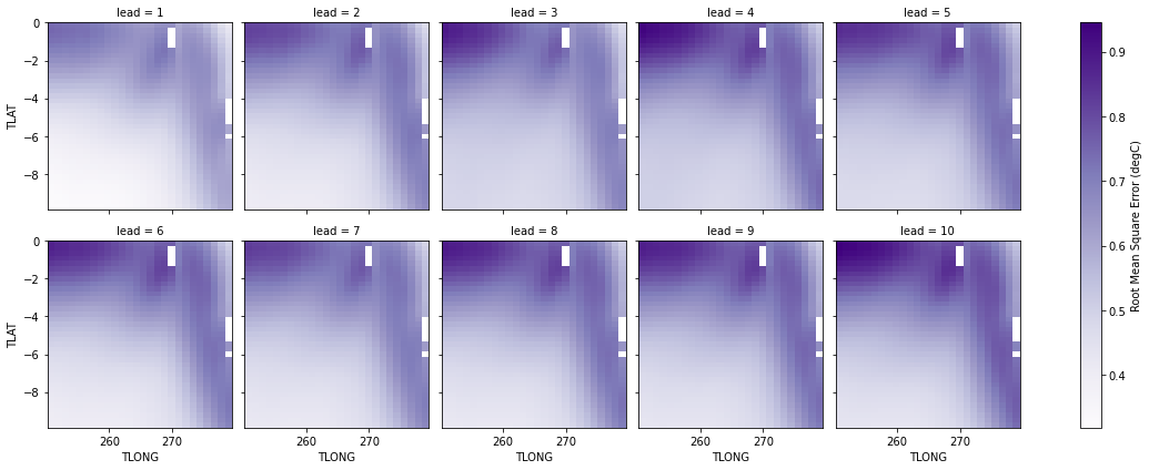
Root Mean Square Error of SSTs

We can also check error in our forecasts, just by changing the metric keyword to _rmse() or _mae().

rmse = hindcast_detrend.verify(
    metric="rmse", comparison="e2o", dim="init", alignment="same_verif"
)

p = rmse.SST.plot.pcolormesh(
    x="TLONG",
    y="TLAT",
    col="lead",
    col_wrap=5,
    cbar_kwargs={"label": "Root Mean Square Error (degC)"},
    cmap="Purples",
)