You can run this notebook in a live session ![]() or view it on Github.
or view it on Github.
Demo of Perfect Model Predictability Functions#
This demo demonstrates climpred’s capabilities for a perfect-model framework ensemble simulation with PerfectModelEnsemble.
What’s a perfect-model framework simulation?
A perfect-model framework uses a set of ensemble simulations that are based on a General Circulation Model (GCM) or Earth System Model (ESM) alone. There is no use of any reanalysis, reconstruction, or data product to initialize the decadal prediction ensemble. An arbitrary number of members are initialized from perturbed initial conditions, and the control simulation can be viewed as just another member, in climpred’s view as member 0.
How to compare predictability skill score:
As no observational data interferes with the random climate evolution of the model, we cannot use an observation-based reference for computing skill scores. Therefore, we can compare the members with one another ("m2m") [Séférian et al., 2018], against the ensemble mean ("m2e") [Griffies and Bryan, 1997], or against the control ("m2c") [Séférian et al., 2018]. We can also compare the ensemble mean to the control member ("e2c") [Griffies and Bryan, 1997]. See comparisons for more information.
When to use perfect-model frameworks:
You don’t have a sufficiently long observational record to use as a reference.
You want to avoid biases between model climatology and reanalysis climatology.
You want to avoid sensitive reactions of biogeochemical cycles to disruptive changes in ocean physics due to assimilation.
You want to delve into process understanding of predictability in a model without outside artifacts.
# linting
%load_ext nb_black
%load_ext lab_black
%matplotlib inline
import matplotlib.pyplot as plt
import numpy as np
import xarray as xr

import climpred
Load sample data
Here we use a subset of ensembles and members from the MPI-ESM-LR (CMIP6 version) esmControl simulation of an early state produce for [Spring and Ilyina, 2020].
1-dimensional output#
Our 1D sample output contains datasets of time series of certain spatially averaged area ('global', 'North_Atlantic') and temporally averaged period (ym, DJF, …) for lead years (1, …, 20).
initialized: The ensemble dataset of all members (1, …, 10), inits (initialization years: 3014, 3023, …, 3257), areas, periods, and lead years.
control: The control dataset with the same areas and periods, as well as the years 3000 to 3299.
# take North Atlantic yearmean
initialized = climpred.tutorial.load_dataset("MPI-PM-DP-1D")
control = climpred.tutorial.load_dataset("MPI-control-1D")
initialized["lead"].attrs = {"units": "years"}
We’ll sub-select annual means ("ym") of sea surface temperature ("tos") in the North Atlantic.
# Add to climpred PerfectModelEnsemble object.
pm = (
    climpred.PerfectModelEnsemble(initialized)
    .add_control(control)
    .sel(area="North_Atlantic", period="ym", drop=True)
)
pm
/Users/aaron.spring/Coding/climpred/climpred/utils.py:191: UserWarning: Assuming annual resolution starting Jan 1st due to numeric inits. Please change ``init`` to a datetime if it is another resolution. We recommend using xr.CFTimeIndex as ``init``, see https://climpred.readthedocs.io/en/stable/setting-up-data.html.
  warnings.warn(
climpred.PerfectModelEnsemble
<Initialized Ensemble>
Dimensions:     (lead: 20, init: 12, member: 10)
Coordinates:
  * lead        (lead) int64 1 2 3 4 5 6 7 8 9 10 11 12 13 14 15 16 17 18 19 20
  * init        (init) object 3014-01-01 00:00:00 ... 3257-01-01 00:00:00
  * member      (member) int64 0 1 2 3 4 5 6 7 8 9
    valid_time  (lead, init) object 3015-01-01 00:00:00 ... 3277-01-01 00:00:00
Data variables:
    tos         (lead, init, member) float32 10.78 10.92 11.11 ... 10.83 10.89
    sos         (lead, init, member) float32 33.38 33.37 33.28 ... 33.4 33.48
AMO (lead, init, member) float32 0.07232 0.1894 ... -0.01757 0.06075- lead: 20
- init: 12
- member: 10
- lead(lead)int641 2 3 4 5 6 7 ... 15 16 17 18 19 20
- units :
- years
- standard_name :
- forecast_period
- long_name :
- Lead
- description :
- Forecast period is the time interval between the forecast reference time and the validity time. A period is an interval of time, or the time-period of an oscillation.
array([ 1, 2, 3, 4, 5, 6, 7, 8, 9, 10, 11, 12, 13, 14, 15, 16, 17, 18, 19, 20]) - init(init)object3014-01-01 00:00:00 ... 3257-01-...
- standard_name :
- forecast_reference_time
- long_name :
- Initialization
- description :
- The forecast reference time in NWP is the "data time", the time of the analysis from which the forecast was made. It is not the time for which the forecast is valid; the standard name of time should be used for that time.
array([cftime.DatetimeProlepticGregorian(3014, 1, 1, 0, 0, 0, 0, has_year_zero=True), cftime.DatetimeProlepticGregorian(3023, 1, 1, 0, 0, 0, 0, has_year_zero=True), cftime.DatetimeProlepticGregorian(3045, 1, 1, 0, 0, 0, 0, has_year_zero=True), cftime.DatetimeProlepticGregorian(3061, 1, 1, 0, 0, 0, 0, has_year_zero=True), cftime.DatetimeProlepticGregorian(3124, 1, 1, 0, 0, 0, 0, has_year_zero=True), cftime.DatetimeProlepticGregorian(3139, 1, 1, 0, 0, 0, 0, has_year_zero=True), cftime.DatetimeProlepticGregorian(3144, 1, 1, 0, 0, 0, 0, has_year_zero=True), cftime.DatetimeProlepticGregorian(3175, 1, 1, 0, 0, 0, 0, has_year_zero=True), cftime.DatetimeProlepticGregorian(3178, 1, 1, 0, 0, 0, 0, has_year_zero=True), cftime.DatetimeProlepticGregorian(3228, 1, 1, 0, 0, 0, 0, has_year_zero=True), cftime.DatetimeProlepticGregorian(3237, 1, 1, 0, 0, 0, 0, has_year_zero=True), cftime.DatetimeProlepticGregorian(3257, 1, 1, 0, 0, 0, 0, has_year_zero=True)], dtype=object) - member(member)int640 1 2 3 4 5 6 7 8 9
- standard_name :
- realization
- long_name :
- Member
- description :
- Realization is used to label a dimension that can be thought of asa statistical sample, e.g., labelling members of a model ensemble.
array([0, 1, 2, 3, 4, 5, 6, 7, 8, 9])
- valid_time(lead, init)object3015-01-01 00:00:00 ... 3277-01-...
- long_name :
- validity time
- standard_name :
- time
- description :
- time for which the forecast is valid
- calculate :
- init + lead
- amip :
- time
array([[cftime.DatetimeProlepticGregorian(3015, 1, 1, 0, 0, 0, 0, has_year_zero=True),
        cftime.DatetimeProlepticGregorian(3024, 1, 1, 0, 0, 0, 0, has_year_zero=True),
        cftime.DatetimeProlepticGregorian(3046, 1, 1, 0, 0, 0, 0, has_year_zero=True),
        cftime.DatetimeProlepticGregorian(3062, 1, 1, 0, 0, 0, 0, has_year_zero=True),
        cftime.DatetimeProlepticGregorian(3125, 1, 1, 0, 0, 0, 0, has_year_zero=True),
        cftime.DatetimeProlepticGregorian(3140, 1, 1, 0, 0, 0, 0, has_year_zero=True),
        cftime.DatetimeProlepticGregorian(3145, 1, 1, 0, 0, 0, 0, has_year_zero=True),
        cftime.DatetimeProlepticGregorian(3176, 1, 1, 0, 0, 0, 0, has_year_zero=True),
        cftime.DatetimeProlepticGregorian(3179, 1, 1, 0, 0, 0, 0, has_year_zero=True),
        cftime.DatetimeProlepticGregorian(3229, 1, 1, 0, 0, 0, 0, has_year_zero=True),
        cftime.DatetimeProlepticGregorian(3238, 1, 1, 0, 0, 0, 0, has_year_zero=True),
        cftime.DatetimeProlepticGregorian(3258, 1, 1, 0, 0, 0, 0, has_year_zero=True)],
       [cftime.DatetimeProlepticGregorian(3016, 1, 1, 0, 0, 0, 0, has_year_zero=True),
        cftime.DatetimeProlepticGregorian(3025, 1, 1, 0, 0, 0, 0, has_year_zero=True),
        cftime.DatetimeProlepticGregorian(3047, 1, 1, 0, 0, 0, 0, has_year_zero=True),
        cftime.DatetimeProlepticGregorian(3063, 1, 1, 0, 0, 0, 0, has_year_zero=True),
        cftime.DatetimeProlepticGregorian(3126, 1, 1, 0, 0, 0, 0, has_year_zero=True),
        cftime.DatetimeProlepticGregorian(3141, 1, 1, 0, 0, 0, 0, has_year_zero=True),
        cftime.DatetimeProlepticGregorian(3146, 1, 1, 0, 0, 0, 0, has_year_zero=True),
        cftime.DatetimeProlepticGregorian(3177, 1, 1, 0, 0, 0, 0, has_year_zero=True),
...
        cftime.DatetimeProlepticGregorian(3158, 1, 1, 0, 0, 0, 0, has_year_zero=True),
        cftime.DatetimeProlepticGregorian(3163, 1, 1, 0, 0, 0, 0, has_year_zero=True),
        cftime.DatetimeProlepticGregorian(3194, 1, 1, 0, 0, 0, 0, has_year_zero=True),
        cftime.DatetimeProlepticGregorian(3197, 1, 1, 0, 0, 0, 0, has_year_zero=True),
        cftime.DatetimeProlepticGregorian(3247, 1, 1, 0, 0, 0, 0, has_year_zero=True),
        cftime.DatetimeProlepticGregorian(3256, 1, 1, 0, 0, 0, 0, has_year_zero=True),
        cftime.DatetimeProlepticGregorian(3276, 1, 1, 0, 0, 0, 0, has_year_zero=True)],
       [cftime.DatetimeProlepticGregorian(3034, 1, 1, 0, 0, 0, 0, has_year_zero=True),
        cftime.DatetimeProlepticGregorian(3043, 1, 1, 0, 0, 0, 0, has_year_zero=True),
        cftime.DatetimeProlepticGregorian(3065, 1, 1, 0, 0, 0, 0, has_year_zero=True),
        cftime.DatetimeProlepticGregorian(3081, 1, 1, 0, 0, 0, 0, has_year_zero=True),
        cftime.DatetimeProlepticGregorian(3144, 1, 1, 0, 0, 0, 0, has_year_zero=True),
        cftime.DatetimeProlepticGregorian(3159, 1, 1, 0, 0, 0, 0, has_year_zero=True),
        cftime.DatetimeProlepticGregorian(3164, 1, 1, 0, 0, 0, 0, has_year_zero=True),
        cftime.DatetimeProlepticGregorian(3195, 1, 1, 0, 0, 0, 0, has_year_zero=True),
        cftime.DatetimeProlepticGregorian(3198, 1, 1, 0, 0, 0, 0, has_year_zero=True),
        cftime.DatetimeProlepticGregorian(3248, 1, 1, 0, 0, 0, 0, has_year_zero=True),
        cftime.DatetimeProlepticGregorian(3257, 1, 1, 0, 0, 0, 0, has_year_zero=True),
        cftime.DatetimeProlepticGregorian(3277, 1, 1, 0, 0, 0, 0, has_year_zero=True)]],
      dtype=object)
- tos(lead, init, member)float3210.78 10.92 11.11 ... 10.83 10.89
array([[[10.781249, 10.917702, ..., 10.897053, 10.843189], [10.727219, 10.813577, ..., 10.803096, 10.651206], ..., [10.294819, 10.539777, ..., 10.442225, 10.412181], [10.385962, 10.594727, ..., 10.409877, 10.403644]], [[11.026904, 10.881209, ..., 10.903457, 10.85706 ], [10.936329, 11.062461, ..., 10.968625, 11.082683], ..., [10.113186, 10.293538, ..., 10.450742, 10.182688], [10.549644, 10.482872, ..., 10.614776, 10.51542 ]], ..., [[10.877393, 10.962437, ..., 10.858264, 10.441303], [10.503685, 10.489896, ..., 11.052794, 10.790496], ..., [10.694736, 10.678864, ..., 10.324147, 10.555562], [10.533122, 10.690272, ..., 10.522203, 11.049645]], [[11.197919, 10.93896 , ..., 10.838304, 10.451338], [10.67775 , 10.550334, ..., 10.607387, 10.692555], ..., [10.642373, 10.502099, ..., 10.11778 , 10.391133], [10.826764, 10.684681, ..., 10.829444, 10.894786]]], dtype=float32) - sos(lead, init, member)float3233.38 33.37 33.28 ... 33.4 33.48
array([[[33.379833, 33.366467, ..., 33.36124 , 33.32225 ], [33.377155, 33.373028, ..., 33.346344, 33.38318 ], ..., [33.217045, 33.2169 , ..., 33.24268 , 33.241886], [33.27586 , 33.298878, ..., 33.232338, 33.308716]], [[33.408016, 33.325253, ..., 33.42898 , 33.345768], [33.3932 , 33.400852, ..., 33.3288 , 33.398758], ..., [33.277046, 33.27699 , ..., 33.328503, 33.218845], [33.33428 , 33.243446, ..., 33.216988, 33.290936]], ..., [[33.39525 , 33.51696 , ..., 33.341 , 33.238438], [33.367573, 33.445225, ..., 33.315975, 33.344593], ..., [33.387165, 33.345234, ..., 33.189358, 33.299137], [33.420033, 33.389782, ..., 33.43263 , 33.552074]], [[33.36968 , 33.55584 , ..., 33.390663, 33.31099 ], [33.402542, 33.388348, ..., 33.343822, 33.431545], ..., [33.246838, 33.30958 , ..., 33.144096, 33.204456], [33.4219 , 33.406277, ..., 33.40383 , 33.48065 ]]], dtype=float32) - AMO(lead, init, member)float320.07232 0.1894 ... -0.01757 0.06075
array([[[ 0.072317,  0.189433, ...,  0.183764,  0.139705],
        [-0.05801 , -0.092494, ...,  0.131268, -0.141136],
        ...,
        [-0.250911, -0.144247, ..., -0.144506, -0.102277],
        [-0.208696, -0.057604, ..., -0.150325, -0.327045]],

       [[ 0.222662,  0.05584 , ...,  0.081747, -0.005777],
        [ 0.085213, -0.02169 , ...,  0.237478,  0.120696],
        ...,
        [-0.239757, -0.290068, ..., -0.190722, -0.152883],
        [-0.283574, -0.091263, ..., -0.003737, -0.199744]],

       ...,

       [[ 0.034137,  0.121907, ...,  0.014317, -0.101567],
        [-0.160837, -0.123508, ...,  0.303377,  0.276406],
        ...,
        [ 0.005184,  0.020541, ..., -0.080405, -0.202475],
        [-0.008904, -0.089735, ..., -0.026045,  0.194669]],

       [[ 0.325681,  0.06963 , ..., -0.17881 , -0.209799],
        [-0.122161,  0.146038, ..., -0.013272,  0.045822],
        ...,
        [ 0.105318, -0.048179, ..., -0.166912, -0.266466],
        [-0.01501 , -0.08603 , ..., -0.017568,  0.060747]]], dtype=float32)
<Control Simulation>
Dimensions:  (time: 300)
Coordinates:
  * time     (time) object 3000-01-01 00:00:00 ... 3299-01-01 00:00:00
Data variables:
    tos      (time) float32 10.91 10.96 10.93 11.12 ... 10.54 10.52 10.59 10.84
    sos      (time) float32 33.45 33.37 33.42 33.44 ... 33.4 33.46 33.39 33.38
AMO (time) float32 0.1678 0.1614 -0.1101 ... 0.01479 -0.02503 0.07905- time: 300
- time(time)object3000-01-01 00:00:00 ... 3299-01-...
- long_name :
- time
- standard_name :
- time
array([cftime.DatetimeProlepticGregorian(3000, 1, 1, 0, 0, 0, 0, has_year_zero=True),
       cftime.DatetimeProlepticGregorian(3001, 1, 1, 0, 0, 0, 0, has_year_zero=True),
       cftime.DatetimeProlepticGregorian(3002, 1, 1, 0, 0, 0, 0, has_year_zero=True),
       ...,
       cftime.DatetimeProlepticGregorian(3297, 1, 1, 0, 0, 0, 0, has_year_zero=True),
       cftime.DatetimeProlepticGregorian(3298, 1, 1, 0, 0, 0, 0, has_year_zero=True),
       cftime.DatetimeProlepticGregorian(3299, 1, 1, 0, 0, 0, 0, has_year_zero=True)],
      dtype=object)
- tos(time)float3210.91 10.96 10.93 ... 10.59 10.84
array([10.906495, 10.958404, 10.93251 , ..., 10.516892, 10.586926, 10.836343], dtype=float32) - sos(time)float3233.45 33.37 33.42 ... 33.39 33.38
array([33.449768, 33.3701 , 33.424828, ..., 33.455902, 33.391457, 33.38208 ], dtype=float32) - AMO(time)float320.1678 0.1614 ... -0.02503 0.07905
array([ 0.167775,  0.161447, -0.110121, ...,  0.01479 , -0.02503 ,  0.079047],
      dtype=float32)
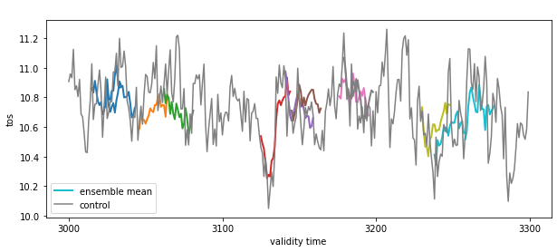
PredictionEnsemble.plot() displays timeseries for 1-dimensional data.
pm.plot()
<AxesSubplot:title={'center':' '}, xlabel='validity time', ylabel='tos'>
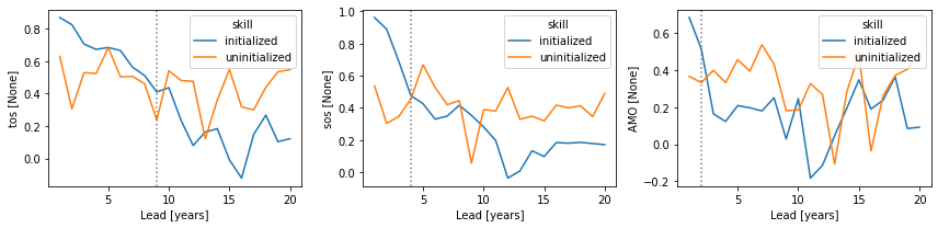
Forecast Verification#
Optionally, PerfectModelEnsemble.verify() (reference=...) verifies against reference forecasts (like "persistence" or "uninitialized").
If uninitialized not present, you can PerfectModelEnsemble.generate_uninitialized() from control.
pm = pm.generate_uninitialized()
from climpred.horizon import horizon

skill = pm.verify(
    metric="acc", comparison="m2e", dim=["init", "member"], reference=["uninitialized"]
)
ph = horizon(skill.sel(skill="initialized") > skill.sel(skill="uninitialized"))
fig, ax = plt.subplots(ncols=3, figsize=(12, 3))
for i, v in enumerate(skill.data_vars):
    fg = skill[v].plot(hue="skill", ax=ax[i])
    # adds gray line at last lead where initialized > uninitialized
    ax[i].axvline(x=ph[v], c="gray", ls=":", label="predictability horizon")
plt.tight_layout()
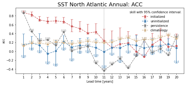
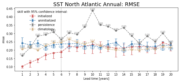
Bootstrapping with Replacement#
Here, we bootstrap the ensemble with replacement [Goddard et al., 2013] to compare the initialized ensemble to an uninitialized counterpart and a persistence reference forecast with PerfectModelEnsemble.bootstrap(). The visualization is based on those used in Li et al. [2016]. The p-value demonstrates the probability that the reference forecasts beat the initialized forecast based on N bootstrapping with replacement.
for metric in ["acc", "rmse"]:
    bootstrapped = pm[["tos"]].bootstrap(
        metric=metric,
        comparison="m2e",
        dim=["init", "member"],
        resample_dim="member",
        iterations=21,
        sig=95,
        reference=["uninitialized", "persistence", "climatology"],
    )

    climpred.graphics.plot_bootstrapped_skill_over_leadyear(bootstrapped)
    # adds gray line where last lead p <= 0.05
    ph = horizon(bootstrapped.sel(results="p", skill="uninitialized") <= 0.05)
    plt.axvline(x=ph.tos, c="gray", ls=":", label="predictability horizon")
    plt.title(
        " ".join(["SST", "North Atlantic", "Annual:", metric.upper()]), fontsize=18
    )
    plt.ylabel(metric)
    plt.show()
Computing Skill with Different Comparison Methods#
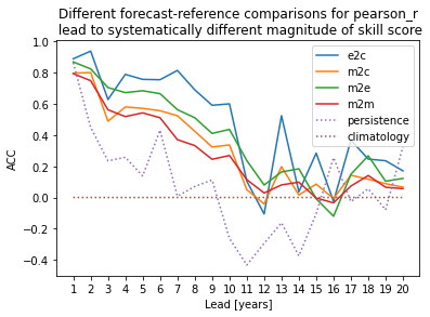
Here, we use PerfectModelEnsemble.verify() to compute the Anomaly Correlation Coefficient (ACC) climpred.metrics._pearson_r() with different comparison methods. This generates different ACC values by design. See comparison for a description of the various ways to compute skill scores for a perfect-model framework.
for c in ["e2c", "m2c", "m2e", "m2m"]:
    dim = "init" if c == "e2c" else ["init", "member"]
    pm.verify(metric="acc", comparison=c, dim=dim)["tos"].plot(label=c)
# Persistence computation for a baseline.
for r in ["persistence", "climatology"]:
    pm.verify(metric="acc", comparison=c, dim=dim, reference=r)["tos"].sel(
        skill=r
    ).plot(label=r, ls=":")
plt.ylabel("ACC")
plt.xticks(np.arange(1, 21))
plt.legend()
plt.title(
    "Different forecast-reference comparisons for pearson_r"
    "\n lead to systematically different magnitude of skill score"
)
plt.show()
3-dimensional output (maps)#
We also have some sample output that contains gridded time series on the curvilinear MPI grid. climpred is indifferent to any dimensions that exist in addition to init, member, and lead. In other words, the functions are set up to make these computations on a grid, if one includes lat, lon, lev, depth, etc.
initialized3d: The ensemble dataset of members (1, … , 4), inits (initialization years: 3014, 3061, 3175, 3237), and lead years (1, …, 5).
control3d: The control dataset spanning (3000, …, 3049).
# Sea surface temperature
initialized3d = climpred.tutorial.load_dataset("MPI-PM-DP-3D")
control3d = climpred.tutorial.load_dataset("MPI-control-3D")

initialized3d["lead"].attrs = {"units": "years"}
# Create climpred PerfectModelEnsemble object.
pm = (
    climpred.PerfectModelEnsemble(initialized3d)
    .add_control(control3d)
    .generate_uninitialized()[["tos"]]
)
/Users/aaron.spring/Coding/climpred/climpred/utils.py:191: UserWarning: Assuming annual resolution starting Jan 1st due to numeric inits. Please change ``init`` to a datetime if it is another resolution. We recommend using xr.CFTimeIndex as ``init``, see https://climpred.readthedocs.io/en/stable/setting-up-data.html.
  warnings.warn(
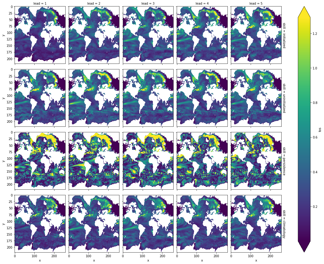
Maps of Skill by Lead Year#
skill = pm.verify(
    metric="mae",
    comparison="m2e",
    dim=["init", "member"],
    reference=["uninitialized", "persistence", "climatology"],
)
skill.tos.plot(col="lead", row="skill", yincrease=False, robust=True)
<xarray.plot.facetgrid.FacetGrid at 0x1464bdc10>
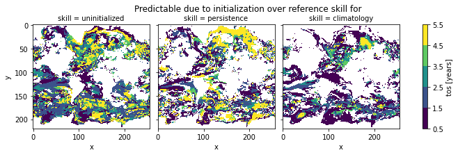
# initialized data has only five leads
ph = horizon(skill.sel(skill="initialized") < skill.drop_sel(skill="initialized"))

ph.tos.plot(yincrease=False, levels=np.arange(0.5, 5.51), col="skill")
plt.suptitle("Predictable due to initialization over reference skill for", y=1.02)
plt.show()
References#
L. Goddard, A. Kumar, A. Solomon, D. Smith, G. Boer, P. Gonzalez, V. Kharin, W. Merryfield, C. Deser, S. J. Mason, B. P. Kirtman, R. Msadek, R. Sutton, E. Hawkins, T. Fricker, G. Hegerl, C. a. T. Ferro, D. B. Stephenson, G. A. Meehl, T. Stockdale, R. Burgman, A. M. Greene, Y. Kushnir, M. Newman, J. Carton, I. Fukumori, and T. Delworth. A verification framework for interannual-to-decadal predictions experiments. Climate Dynamics, 40(1-2):245–272, January 2013. doi:10/f4jjvf.
S. M. Griffies and K. Bryan. A predictability study of simulated North Atlantic multidecadal variability. Climate Dynamics, 13(7-8):459–487, August 1997. doi:10/ch4kc4.
Hongmei Li, Tatiana Ilyina, Wolfgang A. Müller, and Frank Sienz. Decadal predictions of the North Atlantic CO2 uptake. Nature Communications, 7:11076, March 2016. doi:10/f8wkrs.
Aaron Spring and Tatiana Ilyina. Predictability Horizons in the Global Carbon Cycle Inferred From a Perfect-Model Framework. Geophysical Research Letters, 47(9):e2019GL085311, 2020. doi:10/ggtbv2.
Roland Séférian, Sarah Berthet, and Matthieu Chevallier. Assessing the Decadal Predictability of Land and Ocean Carbon Uptake. Geophysical Research Letters, March 2018. doi:10/gdb424.