You can run this notebook in a live session or view it on Github.

Significance Testing

This demo shows how to handle significance testing with HindcastEnsemble.bootstrap() and PerfectModelEnsemble.bootstrap().

# linting
%load_ext nb_black
%load_ext lab_black

import xarray as xr
import numpy as np
from climpred.tutorial import load_dataset
from climpred import HindcastEnsemble, PerfectModelEnsemble
import matplotlib.pyplot as plt

# load data
v = "SST"
hind = load_dataset("CESM-DP-SST")[v]
hind.lead.attrs["units"] = "years"

hist = load_dataset("CESM-LE")[v]
hist = hist - hist.mean()

obs = load_dataset("ERSST")[v]
obs = obs - obs.mean()

hindcast = HindcastEnsemble(hind).add_uninitialized(hist).add_observations(obs)

hindcast.plot()

/Users/aaron.spring/Coding/climpred/climpred/utils.py:191: UserWarning: Assuming annual resolution starting Jan 1st due to numeric inits. Please change ``init`` to a datetime if it is another resolution. We recommend using xr.CFTimeIndex as ``init``, see https://climpred.readthedocs.io/en/stable/setting-up-data.html.
  warnings.warn(
/Users/aaron.spring/Coding/climpred/climpred/utils.py:191: UserWarning: Assuming annual resolution starting Jan 1st due to numeric inits. Please change ``init`` to a datetime if it is another resolution. We recommend using xr.CFTimeIndex as ``init``, see https://climpred.readthedocs.io/en/stable/setting-up-data.html.
  warnings.warn(

<AxesSubplot:xlabel='validity time', ylabel='SST'>

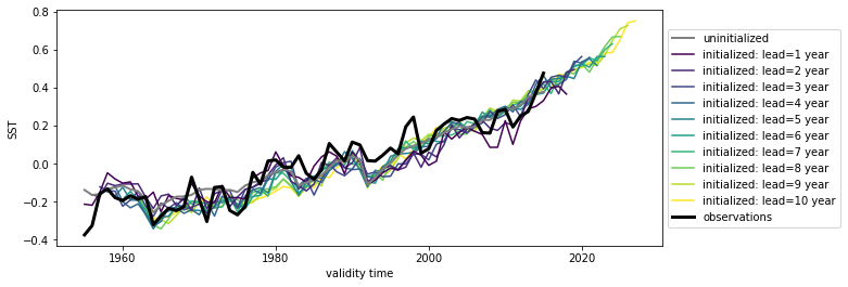
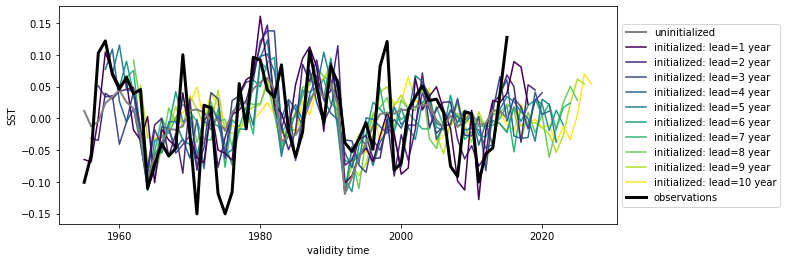
Here we see the strong trend due to climate change. This trend is not linear but rather quadratic. Because we often aim to prediction natural variations and not specifically the external forcing in initialized predictions, we remove the 2nd-order trend from each dataset along a time axis.

from climpred.stats import rm_poly

hindcast = hindcast.map(rm_poly, dim="init_or_time", deg=2)

hindcast.plot()

<AxesSubplot:xlabel='validity time', ylabel='SST'>

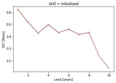
p value for temporal correlations

For correlation metrics the associated p-value checks whether the correlation is significantly different from zero incorporating reduced degrees of freedom due to temporal autocorrelation, see climpred.metrics._pearson_r() and climpred.metrics._pearson_r_eff_p_value().

# level that initialized ensembles are significantly better than other forecast skills
sig = 0.05

acc = hindcast.verify(
    metric="pearson_r", comparison="e2o", dim="init", alignment="same_verif"
)["SST"]
acc_p_value = hindcast.verify(
    metric="pearson_r_eff_p_value", comparison="e2o", dim="init", alignment="same_verif"
)["SST"]

init_color = "indianred"
acc.plot(c=init_color)
acc.where(acc_p_value <= sig).plot(marker="x", c=init_color)

[<matplotlib.lines.Line2D at 0x148ea1970>]

Bootstrapping with replacement

Bootstrapping significance HindcastEnsemble.bootstrap() relies on resampling the underlying data with replacement along resample_dim for a large number of iterations as proposed by the decadal prediction framework of Boer et al. [2016], Goddard et al. [2013].

%%time

bootstrapped_acc = hindcast.bootstrap(
    metric="pearson_r",
    comparison="e2r",
    dim="init",
    alignment="same_verif",
    iterations=500,
    sig=95,
    resample_dim="member",
    reference=["uninitialized", "persistence", "climatology"],
)

CPU times: user 1.12 s, sys: 42.7 ms, total: 1.17 s
Wall time: 1 s

See attributes attrs of the additional dimensions for description.

bootstrapped_acc

<xarray.Dataset>
Dimensions:  (skill: 4, results: 4, lead: 10)
Coordinates:
  * lead     (lead) int32 1 2 3 4 5 6 7 8 9 10
  * results  (results) <U12 'verify skill' 'p' 'low_ci' 'high_ci'
  * skill    (skill) <U13 'initialized' 'uninitialized' ... 'climatology'
Data variables:
    SST      (skill, results, lead) float64 0.6387 0.4999 ... 2.534e-17
Attributes: (12/13)
    prediction_skill_software:     climpred https://climpred.readthedocs.io/
    skill_calculated_by_function:  HindcastEnsemble.bootstrap()
    number_of_initializations:     64
    number_of_members:             10
    alignment:                     same_verif
    metric:                        pearson_r
    ...                            ...
    dim:                           init
    reference:                     ['uninitialized', 'persistence', 'climatol...
    resample_dim:                  member
    sig:                           95
    iterations:                    500
    confidence_interval_levels:    0.975-0.025

# where initialized skill beats reference forecast
init_skill = bootstrapped_acc[v].sel(results="verify skill", skill="initialized")
init_better_than_uninit = init_skill.where(
    bootstrapped_acc[v].sel(results="p", skill="uninitialized") <= sig
)
init_better_than_persistence = init_skill.where(
    bootstrapped_acc[v].sel(results="p", skill="persistence") <= sig
)

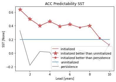
# create a plot by hand
bootstrapped_acc[v].sel(results="verify skill", skill="initialized").plot(
    c=init_color, label="initialized"
)
init_better_than_uninit.plot(
    c=init_color,
    marker="*",
    markersize=15,
    label="initialized better than uninitialized",
)
init_better_than_persistence.plot(
    c=init_color, marker="o", label="initialized better than persistence"
)
bootstrapped_acc[v].sel(results="verify skill", skill="uninitialized").plot(
    c="steelblue", label="uninitialized"
)
bootstrapped_acc[v].sel(results="verify skill", skill="persistence").plot(
    c="gray", label="persistence"
)
plt.title(f"ACC Predictability {v}")
plt.legend(loc="lower right")

<matplotlib.legend.Legend at 0x149c481f0>

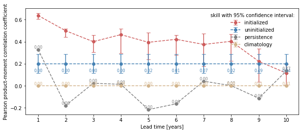
climpred.graphics.plot_bootstrapped_skill_over_leadyear() wraps the above plotting code:

from climpred.graphics import plot_bootstrapped_skill_over_leadyear

plot_bootstrapped_skill_over_leadyear(bootstrapped_acc)

<AxesSubplot:xlabel='Lead time [years]', ylabel='Pearson product-moment correlation coefficient'>

Field significance

Using esmtools.testing.multipletests() to control the false discovery rate (FDR) from the above obtained p-values in geospatial data [Benjamini and Hochberg, 1994, Wilks, 2016].

v = "tos"
ds3d = load_dataset("MPI-PM-DP-3D")[v]
ds3d.lead.attrs["unit"] = "years"
control3d = load_dataset("MPI-control-3D")[v]

pm = PerfectModelEnsemble(ds3d)
pm = pm.add_control(control3d)

/Users/aaron.spring/Coding/climpred/climpred/utils.py:191: UserWarning: Assuming annual resolution starting Jan 1st due to numeric inits. Please change ``init`` to a datetime if it is another resolution. We recommend using xr.CFTimeIndex as ``init``, see https://climpred.readthedocs.io/en/stable/setting-up-data.html.
  warnings.warn(
/Users/aaron.spring/Coding/climpred/climpred/utils.py:191: UserWarning: Assuming annual resolution starting Jan 1st due to numeric inits. Please change ``init`` to a datetime if it is another resolution. We recommend using xr.CFTimeIndex as ``init``, see https://climpred.readthedocs.io/en/stable/setting-up-data.html.
  warnings.warn(

p value for temporal correlations

Lets first calculate the Pearson’s Correlation p-value and then correct afterwards by FDR [Benjamini and Hochberg, 1994].

acc3d = pm.verify(metric="pearson_r", comparison="m2e", dim=["init", "member"])[v]
acc_p_3d = pm.verify(
    metric="pearson_r_p_value", comparison="m2e", dim=["init", "member"]
)[v]

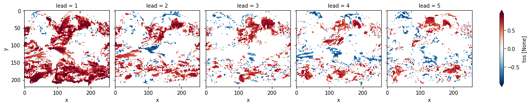
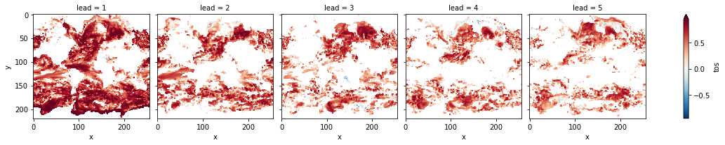
# mask init skill where not significant
acc3d.where(acc_p_3d <= sig).plot(col="lead", robust=True, yincrease=False, x="x")

<xarray.plot.facetgrid.FacetGrid at 0x149eda310>

# apply FDR Benjamini-Hochberg
# relies on esmtools https://github.com/bradyrx/esmtools
from esmtools.testing import multipletests

_, acc_p_3d_fdr_corr = multipletests(acc_p_3d, method="fdr_bh", alpha=sig)

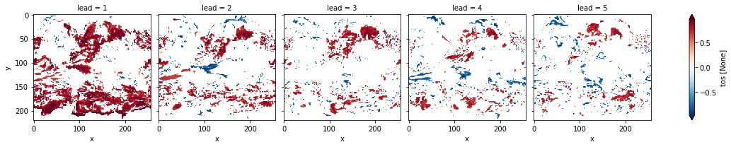
# mask init skill where not significant on corrected p-values
acc3d.where(acc_p_3d_fdr_corr <= sig).plot(
    col="lead", robust=True, yincrease=False, x="x"
)

<xarray.plot.facetgrid.FacetGrid at 0x14994ca30>

# difference due to FDR Benjamini-Hochberg
(acc_p_3d_fdr_corr - acc_p_3d).plot(col="lead", robust=True, yincrease=False, x="x")

<xarray.plot.facetgrid.FacetGrid at 0x149fd1af0>

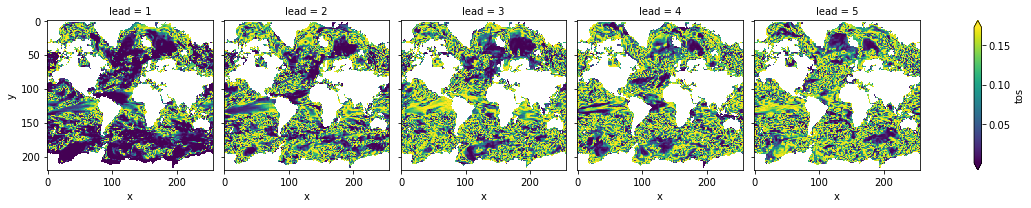
FDR Benjamini-Hochberg increases the p-value and therefore reduces the number of significant grid cells.

Bootstrapping with replacement

The same applies to bootstrapping with replacement in PerfectModelEnsemble.bootstrap(). First calculate the pvalue that uninitialized are better than initialized forecasts. Then correct the FDR [Benjamini and Hochberg, 1994].

%%time
bootstrapped_acc_3d = pm.bootstrap(metric="pearson_r", comparison="m2e", dim=['init', 'member'],
                                   iterations=10, reference='uninitialized')['tos']

/Users/aaron.spring/Coding/climpred/climpred/checks.py:229: UserWarning: Consider chunking input `ds` along other dimensions than needed by algorithm, e.g. spatial dimensions, for parallelized performance increase.
  warnings.warn(

CPU times: user 9.22 s, sys: 2.78 s, total: 12 s
Wall time: 12.3 s

# mask init skill where not significant
bootstrapped_acc_3d.sel(skill="initialized", results="verify skill").where(
    bootstrapped_acc_3d.sel(skill="uninitialized", results="p") <= sig
).plot(col="lead", robust=True, yincrease=False, x="x")

<xarray.plot.facetgrid.FacetGrid at 0x7fc44684d970>

# apply FDR Benjamini-Hochberg
_, bootstrapped_acc_p_3d_fdr_corr = multipletests(
    bootstrapped_acc_3d.sel(skill="uninitialized", results="p"),
    method="fdr_bh",
    alpha=sig,
)

# mask init skill where not significant on corrected p-values
bootstrapped_acc_3d.sel(skill="initialized", results="verify skill").where(
    bootstrapped_acc_p_3d_fdr_corr <= sig * 2
).plot(col="lead", robust=True, yincrease=False, x="x")

<xarray.plot.facetgrid.FacetGrid at 0x7fc44874ce80>

# difference due to FDR Benjamini-Hochberg
(
    bootstrapped_acc_p_3d_fdr_corr
    - bootstrapped_acc_3d.sel(skill="uninitialized", results="p").where(
        bootstrapped_acc_3d.sel(skill="uninitialized", results="p")
    )
).plot(
    col="lead",
    robust=True,
    yincrease=False,
    x="x",
    cmap="RdBu_r",
    vmin=-0.04,
    vmax=0.04,
)

<xarray.plot.facetgrid.FacetGrid at 0x7fc46030d070>

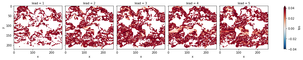
FDR Benjamini-Hochberg increases the p-value and therefore reduces the number of significant grid cells.

Coin test

xskillscore.sign_test() shows which forecast is better. Here we compare the initialized with the uninitialized forecast [DelSole and Tippett, 2016].

skill = hindcast.verify(
    metric="mae",
    comparison="e2o",
    dim=[],
    alignment="same_verif",
    reference="uninitialized",
).SST

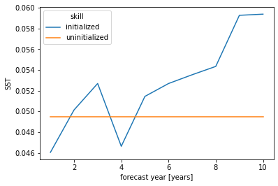
# initialized skill seems clearly better than historical skill for first lead
skill.mean("init").plot(hue="skill")

[<matplotlib.lines.Line2D at 0x7fc2f8fdc370>,
 <matplotlib.lines.Line2D at 0x7fc2f8fdc460>]

from xskillscore import sign_test

# orientation is negative since lower scores are better for MAE
init_better_uninit, walk, confidence = sign_test(
    skill.sel(skill="initialized"),
    skill.sel(skill="uninitialized"),
    time_dim="init",
    orientation="negative",
    alpha=sig,
)

plt.rcParams["legend.loc"] = "upper left"
plt.rcParams["axes.prop_cycle"] = plt.cycler(
    "color", plt.cm.viridis(np.linspace(0, 1, walk.lead.size))
)
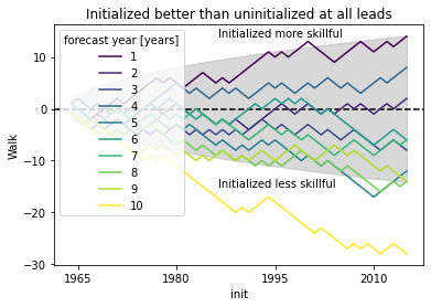
# positive walk means forecast1 (here initialized) is better than forecast2 (uninitialized)
# skillful when colored line above gray line following a random walk
# this gives you the possibility to see which inits have better skill (positive step) than reference
# the final inital init shows the combined result over all inits as the sign_test is a `cumsum`
conf = confidence.isel(lead=0)  # confidence is identical here for all leads
plt.fill_between(conf.init.values, conf, -conf, color="gray", alpha=0.3)
plt.axhline(y=0, c="k", ls="--")
walk.plot(hue="lead")
plt.title("Initialized better than uninitialized at all leads")
plt.ylabel("Walk")
plt.annotate("Initialized more skillful", (-5000, 14), xycoords="data")
plt.annotate("Initialized less skillful", (-5000, -15), xycoords="data")
plt.show()

References

[1] (1,2,3)

Yoav Benjamini and Yosef Hochberg. Controlling the False Discovery Rate: A Practical and Powerful Approach to Multiple Testing. Journal of the Royal Statistical Society: Series B (Methodological), 57(1):13, 1994. doi:10.1111/j.2517-6161.1995.tb02031.x.

[2]

G. J. Boer, D. M. Smith, C. Cassou, F. Doblas-Reyes, G. Danabasoglu, B. Kirtman, Y. Kushnir, M. Kimoto, G. A. Meehl, R. Msadek, W. A. Mueller, K. E. Taylor, F. Zwiers, M. Rixen, Y. Ruprich-Robert, and R. Eade. The Decadal Climate Prediction Project (DCPP) contribution to CMIP6. Geosci. Model Dev., 9(10):3751–3777, October 2016. doi:10/f89qdf.

[3]

Timothy DelSole and Michael K. Tippett. Forecast Comparison Based on Random Walks. Monthly Weather Review, 144(2):615–626, February 2016. doi:10/f782pf.

[4]

L. Goddard, A. Kumar, A. Solomon, D. Smith, G. Boer, P. Gonzalez, V. Kharin, W. Merryfield, C. Deser, S. J. Mason, B. P. Kirtman, R. Msadek, R. Sutton, E. Hawkins, T. Fricker, G. Hegerl, C. a. T. Ferro, D. B. Stephenson, G. A. Meehl, T. Stockdale, R. Burgman, A. M. Greene, Y. Kushnir, M. Newman, J. Carton, I. Fukumori, and T. Delworth. A verification framework for interannual-to-decadal predictions experiments. Climate Dynamics, 40(1-2):245–272, January 2013. doi:10/f4jjvf.

[5]

D. S. Wilks. “The Stippling Shows Statistically Significant Grid Points”: How Research Results are Routinely Overstated and Overinterpreted, and What to Do about It. Bulletin of the American Meteorological Society, 97(12):2263–2273, March 2016. doi:10/f9mvth.