You can run this notebook in a live session or view it on Github.

Diagnosing Potential Predictability

This demo demonstrates climpred’s capabilities to diagnose areas containing potentially predictable variations from a control/verification alone without requiring multi-member, multi-initialization simulations. This notebook identifies the slow components of internal variability that indicate potential predictability. Here, we showcase a set of methods to show regions indicating probabilities for decadal predictability.

# linting
%load_ext nb_black
%load_ext lab_black

%matplotlib inline
import climpred

# Sea surface temperature
varname = "tos"
control3d = climpred.tutorial.load_dataset("MPI-control-3D")[varname].load()

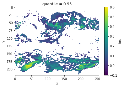
Diagnostic Potential Predictability (DPP)

We can first use the Resplandy et al. [2015] and Séférian et al. [2018] method for computing the unbiased climpred.stats.dpp() by not chunking the time dimension.

# calculate DPP with m=10
DPP10 = climpred.stats.dpp(control3d, m=10, chunk=False)
# calculate a threshold by random shuffling (based on bootstrapping with replacement at 95% significance level)
threshold = climpred.bootstrap.dpp_threshold(
    control3d, m=10, chunk=False, iterations=10, sig=95
)
# plot grid cells where DPP above threshold
DPP10.where(DPP10 > threshold).plot(
    yincrease=False, vmin=-0.1, vmax=0.6, cmap="viridis"
)

<matplotlib.collections.QuadMesh at 0x14b126400>

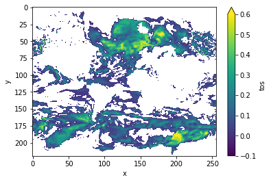
Now, we can turn on chunking (default) to use the Boer [2004] method.

# chunk = True signals the Boer 2004 method
DPP10 = climpred.stats.dpp(control3d, m=10, chunk=True)
threshold = climpred.bootstrap.dpp_threshold(
    control3d, m=10, chunk=True, iterations=10, sig=95
)
DPP10.where(DPP10 > 0).plot(yincrease=False, vmin=-0.1, vmax=0.6, cmap="viridis")

/Users/aaron.spring/anaconda3/envs/climpred-dev/lib/python3.9/site-packages/xarray/core/nputils.py:155: RuntimeWarning: Degrees of freedom <= 0 for slice.
  result = getattr(npmodule, name)(values, axis=axis, **kwargs)
/Users/aaron.spring/anaconda3/envs/climpred-dev/lib/python3.9/site-packages/xarray/core/nputils.py:155: RuntimeWarning: Degrees of freedom <= 0 for slice.
  result = getattr(npmodule, name)(values, axis=axis, **kwargs)

<matplotlib.collections.QuadMesh at 0x14a98c3a0>

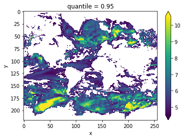
Variance-Weighted Mean Period

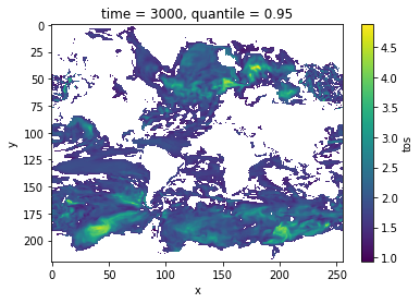
climpred.stats.varweighted_mean_period() uses a periodogram based on a control simulation to extract the mean period of variations, which are weighted by the respective variance. Regions with a high mean period value indicate low-frequency variations with are potentially predictable [Branstator and Teng, 2010].

vwmp = climpred.stats.varweighted_mean_period(control3d, dim="time")
threshold = climpred.bootstrap.varweighted_mean_period_threshold(
    control3d, iterations=10
)
vwmp.where(vwmp > threshold).plot(yincrease=False, robust=True)

<matplotlib.collections.QuadMesh at 0x14b13d160>

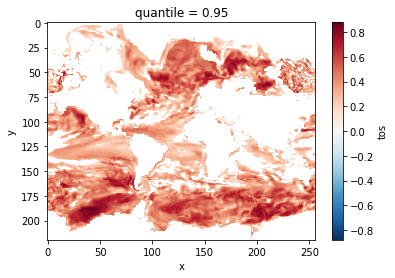
Lag-1 Autocorrelation

The lag-1 autocorrelation also indicates where slower modes of variability occur by identifying regions with high temporal correlation [v Storch and Zwiers, 1999].

from esmtools.stats import autocorr

# use climpred.bootstrap._bootstrap_func to wrap any stats function. `esmtools.stats.autocorr` computes the autocorrelation
# coefficient out to N lags. The first lag is at lag 0, so we select `lead=1`).
threshold = climpred.bootstrap._bootstrap_func(
    autocorr, control3d, nlags=2, resample_dim="time", iterations=10
).isel(lead=1)
corr_ef = autocorr(control3d, nlags=2, dim="time").isel(lead=1)
corr_ef.where(corr_ef > threshold).plot(yincrease=False, robust=False)

<matplotlib.collections.QuadMesh at 0x14a953580>

Decorrelation time

Taking the lagged correlation further over all lags, climpred.stats.decorrelation_time() shows the time after which the autocorrelation fell beyond its e-folding [v Storch and Zwiers, 1999].

threshold = climpred.bootstrap._bootstrap_func(
    climpred.stats.decorrelation_time, control3d, "time", iterations=10
)
decorr_time = climpred.stats.decorrelation_time(control3d)
decorr_time.where(decorr_time > threshold).plot(yincrease=False, robust=False)

<matplotlib.collections.QuadMesh at 0x14a934490>

Verify diagnostic potential predictability in initialized simulations

Do we find predictability in the areas highlighted above also in perfect-model experiments?

ds3d = climpred.tutorial.load_dataset("MPI-PM-DP-3D")[varname]
control3d = climpred.tutorial.load_dataset("MPI-control-3D")[varname]
ds3d["lead"].attrs["units"] = "years"

pm = climpred.PerfectModelEnsemble(ds3d).add_control(control3d)

/Users/aaron.spring/Coding/climpred/climpred/utils.py:191: UserWarning: Assuming annual resolution starting Jan 1st due to numeric inits. Please change ``init`` to a datetime if it is another resolution. We recommend using xr.CFTimeIndex as ``init``, see https://climpred.readthedocs.io/en/stable/setting-up-data.html.
  warnings.warn(
/Users/aaron.spring/Coding/climpred/climpred/utils.py:191: UserWarning: Assuming annual resolution starting Jan 1st due to numeric inits. Please change ``init`` to a datetime if it is another resolution. We recommend using xr.CFTimeIndex as ``init``, see https://climpred.readthedocs.io/en/stable/setting-up-data.html.
  warnings.warn(

bootstrap_skill = pm.bootstrap(
    metric="rmse",
    comparison="m2e",
    dim=["init", "member"],
    reference=["uninitialized"],
    iterations=10,
)

/Users/aaron.spring/Coding/climpred/climpred/checks.py:229: UserWarning: Consider chunking input `ds` along other dimensions than needed by algorithm, e.g. spatial dimensions, for parallelized performance increase.
  warnings.warn(

init_skill = bootstrap_skill.sel(results="verify skill", skill="initialized")
# p value: probability that random uninitialized forecasts perform better than initialized
p = bootstrap_skill.sel(results="p", skill="uninitialized")

init_skill.where(p <= 0.05)[varname].plot(
    col="lead", robust=True, yincrease=False, x="x"
)

<xarray.plot.facetgrid.FacetGrid at 0x14a742d30>

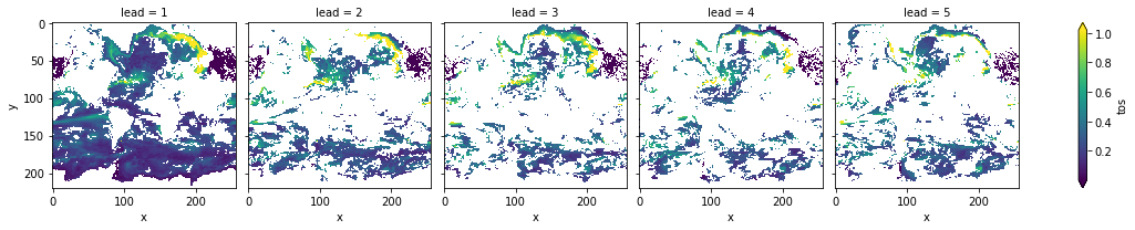
The metric climpred.metrics.__rmse is negatively oriented, e.g. higher values show large disprepancy between members and hence less skill.

As suggested by climpred.stats.dpp(), climpred.stats.varweighted_mean_period() and climpred.stats.decorrelation_time(), there is predictability in the North Atlantic, North Pacific and Southern Ocean in sea-surface temperatures in slight perturbed initialized ensembles .

References

[1]

G. J. Boer. Long time-scale potential predictability in an ensemble of coupled climate models. Climate Dynamics, 23(1):29–44, August 2004. doi:10/csjjbh.

[2]

Grant Branstator and Haiyan Teng. Two Limits of Initial-Value Decadal Predictability in a CGCM. Journal of Climate, 23(23):6292–6311, August 2010. doi:10/bwq92h.

[3]

L. Resplandy, R. Séférian, and L. Bopp. Natural variability of CO2 and O2 fluxes: What can we learn from centuries-long climate models simulations? Journal of Geophysical Research: Oceans, 120(1):384–404, January 2015. doi:10/f63c3h.

[4]

Roland Séférian, Sarah Berthet, and Matthieu Chevallier. Assessing the Decadal Predictability of Land and Ocean Carbon Uptake. Geophysical Research Letters, March 2018. doi:10/gdb424.

[5] (1,2)

H. v Storch and Francis W. Zwiers. Statistical Analysis in Climate Research. Cambridge University Press, Cambridge ; New York, 1999. ISBN 978-0-521-45071-3.