You can run this notebook in a live session or view it on Github.

Implications of `verify(dim)`#

This demo demonstrates how setting dim in PerfectModelEnsemble.verify() and HindcastEnsemble.verify() alters the research question and prediction skill obtained, especially for spatial fields.

What’s the purpose of dim?

dim is designed the same way as in xarray.Dataset.mean(). A given metric is calculated over dimension dim, i.e. the result does not contain dim anymore. dim can be a string or list of strings.

3 ways to calculate aggregated prediction skill

Spatially aggregate first, then verify
verify on each grid point, then aggregate spatially
verify over spatial, member and initialization directly

# linting
%load_ext nb_black
%load_ext lab_black

%matplotlib inline
import matplotlib.pyplot as plt
import numpy as np
import xarray as xr

import climpred

climpred.set_options(PerfectModel_persistence_from_initialized_lead_0=True)

/home/docs/checkouts/readthedocs.org/user_builds/climpred/conda/stable/lib/python3.9/site-packages/tqdm/auto.py:22: TqdmWarning: IProgress not found. Please update jupyter and ipywidgets. See https://ipywidgets.readthedocs.io/en/stable/user_install.html
  from .autonotebook import tqdm as notebook_tqdm

<climpred.options.set_options at 0x7ff320023e50>

sample spatial initialized ensemble data and nomenclature#

We also have some sample output that contains gridded data on MPIOM grid:

initialized3d: The initialized ensemble dataset with
- members (1, … , 4) denoted by $m$
- inits (initialization years: 3014, 3061, 3175, 3237) denoted by $i$
- lead years (1, …, 5) denoted by $l$ .
- x and j (think as longitude and latitude): spatial dimensions denotes by $s$ .
control3d: The control dataset spanning over time (3000, …, 3049) [not used here].

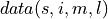In PerfectModelEnsemble.verify(), we calculate a $metric$ on $data(s,i,m,l)$ containing spatial dimensions $s$ and ensemble dimension $i,m,l$ over dimensions $dim$ denoted by $metric(data(s,i,m,l), dim)$ .

# Sea surface temperature
initialized3d = climpred.tutorial.load_dataset("MPI-PM-DP-3D")
control3d = climpred.tutorial.load_dataset("MPI-control-3D")
v = "tos"
initialized3d["lead"].attrs = {"units": "years"}

# Create climpred PerfectModelEnsemble object.
pm = (
    climpred.PerfectModelEnsemble(initialized3d).add_control(control3d)
    # .generate_uninitialized() # needed for uninitialized in reference
)

/home/docs/checkouts/readthedocs.org/user_builds/climpred/checkouts/stable/climpred/utils.py:195: UserWarning: Assuming annual resolution starting Jan 1st due to numeric inits. Please change ``init`` to a datetime if it is another resolution. We recommend using xr.CFTimeIndex as ``init``, see https://climpred.readthedocs.io/en/stable/setting-up-data.html.
  warnings.warn(

/home/docs/checkouts/readthedocs.org/user_builds/climpred/checkouts/stable/climpred/utils.py:195: UserWarning: Assuming annual resolution starting Jan 1st due to numeric inits. Please change ``init`` to a datetime if it is another resolution. We recommend using xr.CFTimeIndex as ``init``, see https://climpred.readthedocs.io/en/stable/setting-up-data.html.
  warnings.warn(

subselecting North Atlantic#

pm = pm.isel(x=slice(80, 150), y=slice(40, 70))
pm.get_initialized().mean(["lead", "member", "init"])[v].plot(
    yincrease=False, robust=True
)

<matplotlib.collections.QuadMesh at 0x7ff2df0ce9d0>

../../_images/2873fd73872cbf7090ed81b27f0a129a4e20263f82f63c388758f583fe36a6ed.png

verify_kwargs = dict(
    metric="pearson_r",  # 'rmse'
    comparison="m2m",
    reference=["persistence", "climatology"],  # "uninitialized",
    skipna=True,
)
dim = ["init", "member"]
spatial_dims = ["x", "y"]

Here, we use the anomaly correlation coefficient climpred.metrics._pearson_r(). Also try root-mean-squared-error climpred.metrics._rmse().

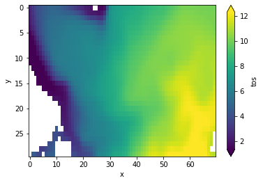
Spatial aggregate first, then `verify`#

Here, we first average the raw ensemble data over the spatial_dims, i.e. creating North Atlantic averaged SST timeseries. On this timeseries, we calculate the prediction skill with PerfectModelEnsemble.verify().

$skill(l) = metric(\overline{data(s,i,m,l)}^s, i, m)$

where $\overline{data}^{dim}$ represents the average of $data$ over dimension $dim$

This approach answers the question: “What’s the prediction skill of SSTs, which were averaged before over the North Atlantic? What is the skill at predicting average [metric] in [domain]?”

Used in Séférian et al. [2018], Spring and Ilyina [2020], Pohlmann et al. [2004].

Recommended by Goddard et al. [2013] section 2.1.4:

“We advocate verifying on at least two spatial scales: (1) the observational grid scales to which the model data is interpolated, and (2) smoothed or regional scales. The latter can be accomplished by suitable spatial-smoothing algorithms, such as simple averages or spectral filters.”

pm_aggregated = pm.mean(spatial_dims)
# see the NA SST timeseries
pm_aggregated.plot(show_members=True)

---------------------------------------------------------------------------
TypeError                                 Traceback (most recent call last)
Cell In [7], line 3
      1 pm_aggregated = pm.mean(spatial_dims)
      2 # see the NA SST timeseries
----> 3 pm_aggregated.plot(show_members=True)

File ~/checkouts/readthedocs.org/user_builds/climpred/checkouts/stable/climpred/classes.py:486, in PredictionEnsemble.plot(self, variable, ax, show_members, cmap, x)
    484 if cmap is None:
    485     cmap = "tab10"
--> 486 return plot_ensemble_perfect_model(
    487     self, variable=variable, ax=ax, show_members=show_members, cmap=cmap
    488 )

File ~/checkouts/readthedocs.org/user_builds/climpred/checkouts/stable/climpred/graphics.py:377, in plot_ensemble_perfect_model(pm, variable, ax, show_members, cmap, x)
    373         dsu.mean("member").plot(
    374             ax=ax, x=x, color=control_color, lw=2, zorder=9, alpha=0.6
    375         )
    376     # plot ensemble mean, first white then color to highlight ensemble mean
--> 377     dsi.mean("member").plot(ax=ax, x=x, color="white", lw=3, zorder=10)
    378     dsi.mean("member").plot(ax=ax, x=x, color=_cmap(ii), lw=2, zorder=11)
    379 dsi.plot(
    380     ax=ax,
    381     x=x,
   (...)
    386     label=labelstr,
    387 )

File ~/checkouts/readthedocs.org/user_builds/climpred/conda/stable/lib/python3.9/site-packages/xarray/plot/accessor.py:46, in DataArrayPlotAccessor.__call__(self, **kwargs)
     44 @functools.wraps(dataarray_plot.plot, assigned=("__doc__", "__annotations__"))
     45 def __call__(self, **kwargs) -> Any:
---> 46     return dataarray_plot.plot(self._da, **kwargs)

File ~/checkouts/readthedocs.org/user_builds/climpred/conda/stable/lib/python3.9/site-packages/xarray/plot/dataarray_plot.py:312, in plot(darray, row, col, col_wrap, ax, hue, subplot_kws, **kwargs)
    308     plotfunc = hist
    310 kwargs["ax"] = ax
--> 312 return plotfunc(darray, **kwargs)

File ~/checkouts/readthedocs.org/user_builds/climpred/conda/stable/lib/python3.9/site-packages/xarray/plot/dataarray_plot.py:517, in line(darray, row, col, figsize, aspect, size, ax, hue, x, y, xincrease, yincrease, xscale, yscale, xticks, yticks, xlim, ylim, add_legend, _labels, *args, **kwargs)
    513 ylabel = label_from_attrs(yplt, extra=y_suffix)
    515 _ensure_plottable(xplt_val, yplt_val)
--> 517 primitive = ax.plot(xplt_val, yplt_val, *args, **kwargs)
    519 if _labels:
    520     if xlabel is not None:

File ~/checkouts/readthedocs.org/user_builds/climpred/conda/stable/lib/python3.9/site-packages/matplotlib/axes/_axes.py:1664, in Axes.plot(self, scalex, scaley, data, *args, **kwargs)
   1662 lines = [*self._get_lines(*args, data=data, **kwargs)]
   1663 for line in lines:
-> 1664     self.add_line(line)
   1665 if scalex:
   1666     self._request_autoscale_view("x")

File ~/checkouts/readthedocs.org/user_builds/climpred/conda/stable/lib/python3.9/site-packages/matplotlib/axes/_base.py:2340, in _AxesBase.add_line(self, line)
   2337 if line.get_clip_path() is None:
   2338     line.set_clip_path(self.patch)
-> 2340 self._update_line_limits(line)
   2341 if not line.get_label():
   2342     line.set_label(f'_child{len(self._children)}')

File ~/checkouts/readthedocs.org/user_builds/climpred/conda/stable/lib/python3.9/site-packages/matplotlib/axes/_base.py:2363, in _AxesBase._update_line_limits(self, line)
   2359 def _update_line_limits(self, line):
   2360     """
   2361     Figures out the data limit of the given line, updating self.dataLim.
   2362     """
-> 2363     path = line.get_path()
   2364     if path.vertices.size == 0:
   2365         return

File ~/checkouts/readthedocs.org/user_builds/climpred/conda/stable/lib/python3.9/site-packages/matplotlib/lines.py:1031, in Line2D.get_path(self)
   1029 """Return the `~matplotlib.path.Path` associated with this line."""
   1030 if self._invalidy or self._invalidx:
-> 1031     self.recache()
   1032 return self._path

File ~/checkouts/readthedocs.org/user_builds/climpred/conda/stable/lib/python3.9/site-packages/matplotlib/lines.py:659, in Line2D.recache(self, always)
    657 if always or self._invalidx:
    658     xconv = self.convert_xunits(self._xorig)
--> 659     x = _to_unmasked_float_array(xconv).ravel()
    660 else:
    661     x = self._x

File ~/checkouts/readthedocs.org/user_builds/climpred/conda/stable/lib/python3.9/site-packages/matplotlib/cbook/__init__.py:1369, in _to_unmasked_float_array(x)
   1367     return np.ma.asarray(x, float).filled(np.nan)
   1368 else:
-> 1369     return np.asarray(x, float)

TypeError: float() argument must be a string or a number, not 'cftime._cftime.DatetimeProlepticGregorian'

../../_images/d0b8395ecb0fbc3f8d1506cd501c90aea82f847e36587c25754ec0bd7e0e5e26.png

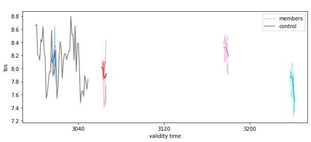
pm_aggregated_skill = pm_aggregated.verify(dim=dim, **verify_kwargs)
pm_aggregated_skill[v].plot(hue="skill")

/Users/aaron.spring/Coding/climpred/climpred/classes.py:1597: UserWarning: Calculate persistence from lead=1 instead of lead=0 (recommended).
  warnings.warn(

[<matplotlib.lines.Line2D at 0x14d4628f0>,
 <matplotlib.lines.Line2D at 0x14d4631c0>,
 <matplotlib.lines.Line2D at 0x14b69cf10>]

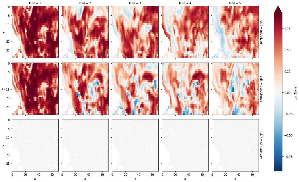
../../_images/1053bc5614e0df55ef1903fb660a50f52250dff35a9298524ec0d5955df86ec5.png

`verify` on each grid point, then aggregate#

Here, we first calculate prediction skill with PerfectModelEnsemble.verify() and then average the SST skill over the North Atlantic region.

$skill(l) = \overline{metric(data(s,i,m,l), i, m)}^s$

This approach answers the question: “What’s the prediction skill of North Altantic SST grid points averaged afterwards? What is the average skill of predicting [metric] in [domain]?”

Used in Frölicher et al. [2020].

grid_point_skill = pm.verify(dim=dim, **verify_kwargs)
grid_point_skill[v].plot(col="lead", row="skill", robust=True, yincrease=False)

/Users/aaron.spring/Coding/climpred/climpred/classes.py:1597: UserWarning: Calculate persistence from lead=1 instead of lead=0 (recommended).
  warnings.warn(

<xarray.plot.facetgrid.FacetGrid at 0x14d8f1180>

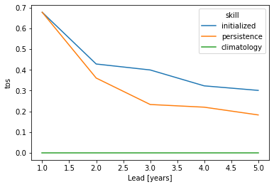
../../_images/f8b86988eb5a90c81dc67c201ea48e776c70aff969a9c3f961aa74d312a6df70.png

grid_point_skill_aggregated = grid_point_skill.mean(spatial_dims)
grid_point_skill_aggregated[v].plot(hue="skill")
plt.show()

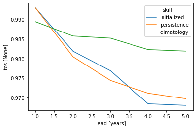
../../_images/61a970f976f6f65ff7e4ea057cc2838a0c08b4749d8781208f80f6b951a2e84c.png

`verify` over each grid point, `member` and `init`ialization directly#

Here, we directly calculate prediction skill with PerfectModelEnsemble.verify() over spatial_dims, member and init.

$skill(l) = metric(data(s,i,m,l), s, i, m)$

This approach answers the question: What’s the prediction skill of the North Atlantic SST pattern (calculated over all members and inits)? What is the spatial skill of predicting [metric] over [domain]?

Used in Becker et al. [2014], Fransner et al. [2020].

skill_all_at_once = pm.verify(dim=dim + spatial_dims, **verify_kwargs)
skill_all_at_once[v].plot(hue="skill")
plt.show()

/Users/aaron.spring/Coding/climpred/climpred/classes.py:1597: UserWarning: Calculate persistence from lead=1 instead of lead=0 (recommended).
  warnings.warn(

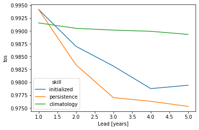
../../_images/8b4407ee21c3be349ce196900df4fbc1e3fc53a06e2d1f802b5763136a3fa903.png

This approach yields very similar results to first calculating prediction skill over the spatial_dims, i.e. calculating a pattern correlation and then doing a mean over ensemble dimensions member and init.

$skill(l) = \overline{metric(data(s,i,m,l), s)}^{i,m}$

skill_spatial_then_ensemble_mean = pm.verify(dim=spatial_dims, **verify_kwargs).mean(
    dim
)
skill_spatial_then_ensemble_mean[v].plot(hue="skill")
plt.show()

/Users/aaron.spring/Coding/climpred/climpred/classes.py:1597: UserWarning: Calculate persistence from lead=1 instead of lead=0 (recommended).
  warnings.warn(

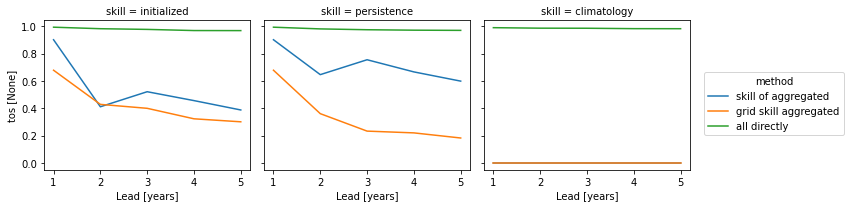
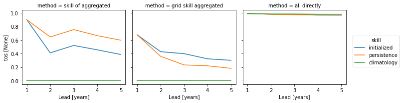
../../_images/b29204c56dc302acd39eb7383de883542c53d68ef5f90a85520575b7031fee72.png

Summary#

The three approaches yield very different results based on the dim keyword. Make you choose dim according to the question you want to answer. And always compare your initialized skill to the reference skills, which also heavily depend on dim. The small details matter a lot!

skills = xr.concat(
    [pm_aggregated_skill, grid_point_skill_aggregated, skill_all_at_once], "method"
).assign_coords(method=["skill of aggregated", "grid skill aggregated", "all directly"])

skills[v].plot(hue="method", col="skill")

<xarray.plot.facetgrid.FacetGrid at 0x14d7f4460>

../../_images/42fa124b97b90a715bc623938ff7659b97ba8ccc0ec26904269871e05873179e.png

skills[v].plot(col="method", hue="skill")

<xarray.plot.facetgrid.FacetGrid at 0x14df5b970>

../../_images/2aceca4e8268e806aafe370f74fc7a7e35bb44650fcbde9a11fb0a313d7c6032.png

References#

1: Emily Becker, Huug van den Dool, and Qin Zhang. Predictability and Forecast Skill in NMME. Journal of Climate, 27(15):5891–5906, August 2014. doi:10.1175/JCLI-D-13-00597.1.
2: Filippa Fransner, François Counillon, Ingo Bethke, Jerry Tjiputra, Annette Samuelsen, Aleksi Nummelin, and Are Olsen. Ocean Biogeochemical Predictions—Initialization and Limits of Predictability. Frontiers in Marine Science, 2020. doi:10/gg22rr.
3: Thomas L. Frölicher, Luca Ramseyer, Christoph C. Raible, Keith B. Rodgers, and John Dunne. Potential predictability of marine ecosystem drivers. Biogeosciences, 17(7):2061–2083, April 2020. doi:10/ggr9mb.
4: L. Goddard, A. Kumar, A. Solomon, D. Smith, G. Boer, P. Gonzalez, V. Kharin, W. Merryfield, C. Deser, S. J. Mason, B. P. Kirtman, R. Msadek, R. Sutton, E. Hawkins, T. Fricker, G. Hegerl, C. a. T. Ferro, D. B. Stephenson, G. A. Meehl, T. Stockdale, R. Burgman, A. M. Greene, Y. Kushnir, M. Newman, J. Carton, I. Fukumori, and T. Delworth. A verification framework for interannual-to-decadal predictions experiments. Climate Dynamics, 40(1-2):245–272, January 2013. doi:10/f4jjvf.
5: Holger Pohlmann, Michael Botzet, Mojib Latif, Andreas Roesch, Martin Wild, and Peter Tschuck. Estimating the Decadal Predictability of a Coupled AOGCM. Journal of Climate, 17(22):4463–4472, November 2004. doi:10/d2qf62.
6: Aaron Spring and Tatiana Ilyina. Predictability Horizons in the Global Carbon Cycle Inferred From a Perfect-Model Framework. Geophysical Research Letters, 47(9):e2019GL085311, 2020. doi:10/ggtbv2.
7: Roland Séférian, Sarah Berthet, and Matthieu Chevallier. Assessing the Decadal Predictability of Land and Ocean Carbon Uptake. Geophysical Research Letters, March 2018. doi:10/gdb424.

climpred documentation

Implications of verify(dim)

Contents

Implications of `verify(dim)`#

sample spatial initialized ensemble data and nomenclature#

subselecting North Atlantic#

Spatial aggregate first, then `verify`#

`verify` on each grid point, then aggregate#

`verify` over each grid point, `member` and `init`ialization directly#

Summary#

References#

climpred documentation

Implications of verify(dim)

Contents

Implications of verify(dim)#

sample spatial initialized ensemble data and nomenclature#

subselecting North Atlantic#

Spatial aggregate first, then verify#

verify on each grid point, then aggregate#

verify over each grid point, member and initialization directly#

Summary#

References#

Implications of `verify(dim)`#

Spatial aggregate first, then `verify`#

`verify` on each grid point, then aggregate#

`verify` over each grid point, `member` and `init`ialization directly#