Hindcast Predictions of Equatorial Pacific SSTs¶

In this example, we evaluate hindcasts (retrospective forecasts) of sea surface temperatures in the eastern equatorial Pacific from CESM-DPLE. These hindcasts are evaluated against a forced ocean–sea ice simulation that initializes the model.

See the quick start for an analysis of time series (rather than maps) from a hindcast prediction ensemble.

[1]:

import warnings

import cartopy.crs as ccrs  # you may need to install cartopy, if not using climpred-dev
import cartopy.feature as cfeature
%matplotlib inline
import matplotlib.pyplot as plt
import numpy as np

import climpred
from climpred import HindcastEnsemble

warnings.filterwarnings("ignore")

We’ll load in a small region of the eastern equatorial Pacific for this analysis example.

[2]:

hind = climpred.tutorial.load_dataset('CESM-DP-SST-3D')['SST']
recon = climpred.tutorial.load_dataset('FOSI-SST-3D')['SST']
hind

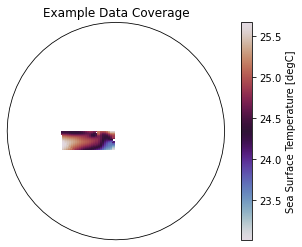
These two example products cover a small portion of the eastern equatorial Pacific.

[3]:

ax = plt.axes(projection=ccrs.Orthographic(-80, 0))
p = ax.pcolormesh(recon.TLONG, recon.TLAT, recon.mean('time'),
              transform=ccrs.PlateCarree(), cmap='twilight')
# ax.add_feature(cfeature.LAND, color='#d3d3d3')
ax.set_global()
plt.colorbar(p, label='Sea Surface Temperature [degC]')
ax.set(title='Example Data Coverage')
plt.show()

../../_images/examples_decadal_tropical-pacific-ssts_5_0.png

It is generally advisable to do all bias correction before instantiating a HindcastEnsemble. However, HindcastEnsemble can also be modified.

climpred requires that lead dimension has an attribute called units indicating what time units the lead is assocated with. Options are: years, seasons, months, weeks, pentads, days. For the this data, the lead units are years.

[4]:

hind['lead'].attrs['units'] = 'years'

[19]:

hindcast = HindcastEnsemble(hind)
hindcast = hindcast.add_observations(recon)
print(hindcast)

climpred.HindcastEnsemble

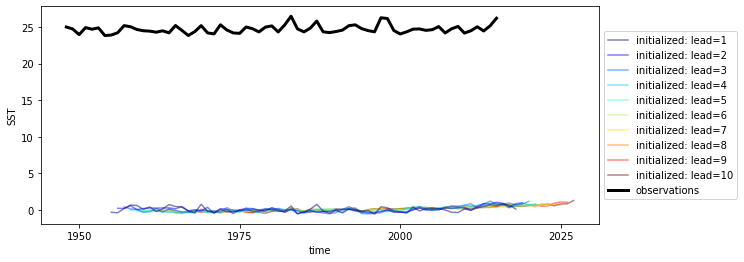
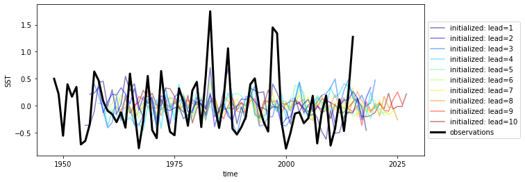
[6]:

# Quick look at the HindEnsemble timeseries: only works for 1-dimensional data, therefore take spatial mean
hindcast.mean(['nlat', 'nlon']).plot()

[6]:

<AxesSubplot:xlabel='time', ylabel='SST'>

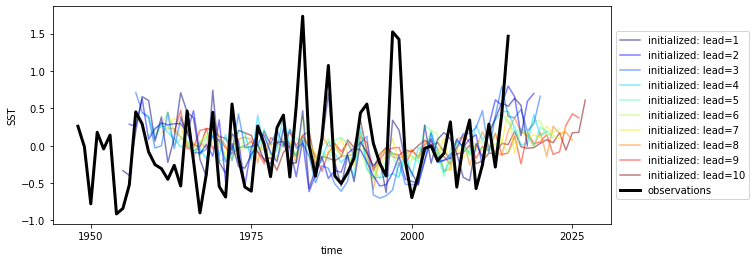
../../_images/examples_decadal_tropical-pacific-ssts_10_1.png

We first need to remove the same climatology that was used to drift-correct the CESM-DPLE.

[10]:

recon = recon - recon.sel(time=slice(1964,2014)).mean('time')
hindcast = hindcast.add_observations(recon)
hindcast.mean(['nlat', 'nlon']).plot()

[10]:

<AxesSubplot:xlabel='time', ylabel='SST'>

../../_images/examples_decadal_tropical-pacific-ssts_12_1.png

We’ll also detrend the reconstruction over its time dimension and initialized forecast ensemble over lead.

[20]:

from esmtools.stats import rm_trend

hindcast_detrend = hindcast.map(rm_trend, dim='lead').map(rm_trend, dim='time')

[21]:

hindcast_detrend.mean(['nlat', 'nlon']).plot()

[21]:

<AxesSubplot:xlabel='time', ylabel='SST'>

../../_images/examples_decadal_tropical-pacific-ssts_15_1.png

Although functions can be called directly in climpred, we suggest that you use our classes (HindcastEnsemble and PerfectModelEnsemble) to make analysis code cleaner.

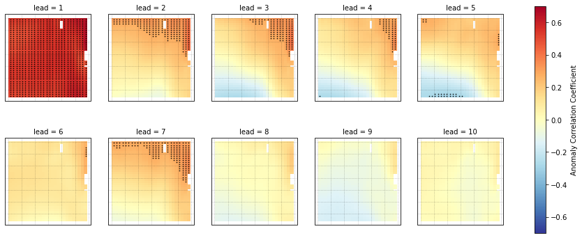
Anomaly Correlation Coefficient of SSTs¶

We can now compute the ACC over all leads and all grid cells.

[13]:

predictability = hindcast_detrend.verify(metric='acc', comparison='e2o', dim='init', alignment='same_verif')
print(predictability)

<xarray.Dataset>
Dimensions:  (lead: 10, nlat: 37, nlon: 26, skill: 1)
Coordinates:
  * lead     (lead) int32 1 2 3 4 5 6 7 8 9 10
    TLONG    (nlat, nlon) float64 250.8 251.9 253.1 254.2 ... 276.7 277.8 278.9
    TAREA    (nlat, nlon) float64 3.661e+13 3.661e+13 ... 3.714e+13 3.714e+13
  * skill    (skill) <U4 'init'
Dimensions without coordinates: nlat, nlon
Data variables:
    SST      (lead, nlat, nlon) float64 0.5079 0.5049 0.5024 ... 0.0701 0.08838

We use the pval keyword to get associated p-values for our ACCs. We can then mask our final maps based on $\alpha = 0.05$ .

[14]:

significance = hindcast_detrend.verify(metric='p_pval', comparison='e2o', dim='init', alignment='same_verif')
# FIX: add missing coords to results
significance.coords['TLAT'] = hind['TLAT']
predictability.coords['TLAT'] = hind['TLAT']

[15]:

# Mask latitude and longitude by significance for stippling.
siglat = significance.TLAT.where(significance.SST <= 0.05)
siglon = significance.TLONG.where(significance.SST <= 0.05)

[16]:

p = predictability.SST.plot.pcolormesh(x='TLONG', y='TLAT',
                                       transform=ccrs.PlateCarree(),
                                       col='lead', col_wrap=5,
                                       subplot_kws={'projection': ccrs.PlateCarree(),
                                                    'aspect': 3},
                                       cbar_kwargs={'label': 'Anomaly Correlation Coefficient'},
                                       vmin=-0.7, vmax=0.7,
                                       cmap='RdYlBu_r')
for i, ax in enumerate(p.axes.flat):
#     ax.add_feature(cfeature.LAND, color='#d3d3d3', zorder=4)
    ax.gridlines(alpha=0.3, color='k', linestyle=':')
    # Add significance stippling
    ax.scatter(siglon.isel(lead=i),
               siglat.isel(lead=i),
               color='k',
               marker='.',
               s=1.5,
               transform=ccrs.PlateCarree())

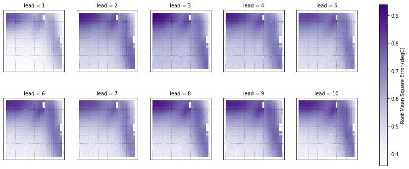
../../_images/examples_decadal_tropical-pacific-ssts_22_0.png

Root Mean Square Error of SSTs¶

We can also check error in our forecasts, just by changing the metric keyword.

[17]:

rmse = hindcast_detrend.verify(metric='rmse', comparison='e2o', dim='init', alignment='same_verif')
rmse.coords['TLAT'] = hind['TLAT']

[18]:

p = rmse.SST.plot.pcolormesh(x='TLONG', y='TLAT',
                            transform=ccrs.PlateCarree(),
                            col='lead', col_wrap=5,
                            subplot_kws={'projection': ccrs.PlateCarree(),
                                        'aspect': 3},
                            cbar_kwargs={'label': 'Root Mean Square Error (degC)'},
                            cmap='Purples')
for ax in p.axes.flat:
#     ax.add_feature(cfeature.LAND, color='#d3d3d3', zorder=4)
    ax.gridlines(alpha=0.3, color='k', linestyle=':')

../../_images/examples_decadal_tropical-pacific-ssts_25_0.png