PredictionEnsemble Objects
One of the major features of climpred is our objects that are based upon the PredictionEnsemble class. We supply users with a HindcastEnsemble and PerfectModelEnsemble object. We encourage users to take advantage of these high-level objects, which wrap all of our core functions.
Briefly, we consider a HindcastEnsemble to be one that is initialized from some observational-like product (e.g., assimilated data, reanalysis products, or a model reconstruction). Thus, this object is built around comparing the initialized ensemble to various observational products. In contrast, a PerfectModelEnsemble is one that is initialized off of a model control simulation. These forecasting systems are not meant to be compared directly to real-world observations. Instead, they
provide a contained model environment with which to theoretically study the limits of predictability. You can read more about the terminology used in climpred here.
Let’s create a demo object to explore some of the functionality and why they are much smoother to use than direct function calls.
[1]:
%matplotlib inline
import matplotlib.pyplot as plt
import xarray as xr

from climpred import HindcastEnsemble, PerfectModelEnsemble
from climpred.tutorial import load_dataset
import climpred

xr.set_options(display_style='text')
[1]:
<xarray.core.options.set_options at 0x7f9590d832e8>
We can now pull in some sample data that is packaged with climpred.
HindcastEnsemble
We’ll start out with a HindcastEnsemble demo, followed by a PerfectModelEnsemble case.
[2]:
hind = climpred.tutorial.load_dataset('CESM-DP-SST') # CESM-DPLE hindcast ensemble output.
obs = climpred.tutorial.load_dataset('ERSST') # ERSST observations.
We need to add a “units” attribute to the hindcast ensemble so that climpred knows how to interpret the lead units.
[3]:
hind["lead"].attrs["units"] = "years"
Now we instantiate the HindcastEnsemble object and append all of our products to it.
[4]:
hindcast = HindcastEnsemble(hind) # Instantiate object by passing in our initialized ensemble.
print(hindcast)
<climpred.HindcastEnsemble>
Initialized Ensemble:
    SST      (init, lead, member) float64 ...
Observations:
    None
Uninitialized:
    None
/Users/aaron.spring/Coding/climpred/climpred/utils.py:141: UserWarning: Assuming annual resolution due to numeric inits. Change init to a datetime if it is another resolution.
  "Assuming annual resolution due to numeric inits. "
Now we just use the add_ methods to attach other objects. See the API here. Note that we strive to make our conventions follow those of ``xarray``’s. For example, we don’t allow inplace operations. One has to run hindcast = hindcast.add_observations(...) to modify the object upon later calls rather than just hindcast.add_observations(...).
[5]:
hindcast = hindcast.add_observations(obs)
print(hindcast)
<climpred.HindcastEnsemble>
Initialized Ensemble:
    SST      (init, lead, member) float64 ...
Observations:
    SST      (time) float32 ...
Uninitialized:
    None
You can apply most standard xarray functions directly to our objects! climpred will loop through the objects and apply the function to all applicable xarray.Datasets within the object. If you reference a dimension that doesn’t exist for the given xarray.Dataset, it will ignore it. This is useful, since the initialized ensemble is expected to have dimension init, while other products have dimension time (see more here).
Let’s start by taking the ensemble mean of the initialized ensemble so our metric computations don’t have to take the extra time on that later. I’m just going to use deterministic metrics here, so we don’t need the individual ensemble members. Note that above our initialized ensemble had a member dimension, and now it is reduced.
[6]:
hindcast = hindcast.mean('member')
hindcast
[6]:
<climpred.HindcastEnsemble>
Initialized Ensemble:
    SST      (init, lead) float64 -0.2121 -0.1637 -0.1206 ... 0.7286 0.7532
Observations:
    SST      (time) float32 ...
Uninitialized:
    None
Arithmetic Operations with PredictionEnsemble Objects
PredictionEnsemble objects support arithmetic operations, i.e., +, -, /, *. You can perform these operations on a HindcastEnsemble or PerfectModelEnsemble by pairing the operation with an int, float, np.ndarray, xr.DataArray, xr.Dataset, or with another PredictionEnsemble object.
An obvious application would be to area-weight an initialized ensemble and all of its associated datasets (like verification products) simultaneously.
[7]:
dple3d = climpred.tutorial.load_dataset('CESM-DP-SST-3D')
verif3d = climpred.tutorial.load_dataset('FOSI-SST-3D')
area = dple3d['TAREA']
Here, we load in a subset of CESM-DPLE over the eastern tropical Pacific. The file includes TAREA, which describes the area of each cell on the curvilinear mesh.
[8]:
hindcast3d = HindcastEnsemble(dple3d)
hindcast3d = hindcast3d.add_observations(verif3d)
hindcast3d
/Users/aaron.spring/Coding/climpred/climpred/utils.py:141: UserWarning: Assuming annual resolution due to numeric inits. Change init to a datetime if it is another resolution.
  "Assuming annual resolution due to numeric inits. "
[8]:
<climpred.HindcastEnsemble>
Initialized Ensemble:
    SST      (init, lead, nlat, nlon) float32 ...
Observations:
    SST      (time, nlat, nlon) float32 ...
Uninitialized:
    None
Now we can perform an area-weighting operation with the HindcastEnsemble object and the area DataArray. climpred cycles through all of the datasets appended to the HindcastEnsemble and applies them. You can see below that the dimensionality is reduced to single time series without spatial information.
[9]:
hindcast3d_aw = (hindcast3d*area).sum(['nlat', 'nlon']) / area.sum(['nlat', 'nlon'])
hindcast3d_aw
[9]:
<climpred.HindcastEnsemble>
Initialized Ensemble:
    SST      (init, lead) float64 -0.3539 0.1947 0.3623 ... 0.662 1.016 1.249
Observations:
    SST      (time) float64 24.76 24.48 23.73 24.68 ... 24.78 24.21 24.92 25.95
Uninitialized:
    None
NOTE: Be careful with the arithmetic operations. Some of the behavior can be unexpected in combination with the fact that generic xarray methods can be applied to climpred objects. For instance, one might be interested in removing a climatology from the verification data to move it to anomaly space. It’s safest to do anything like climatology removal before constructing climpred objects.
Naturally, they would remove some climatology time slice as we do here below. However, note that in the below example, the intialized ensemble returns all zeroes for SST. The reasoning here is that when hindcast.sel(time=...) is called, climpred only applies that slicing to datasets that include the time dimension. Thus, it skips the initialized ensemble and returns the original dataset untouched. This feature is advantageous for cases like hindcast.mean('member'), where it
takes the ensemble mean in all cases that ensemble members exist. So when it performs hindcast - hindcast.sel(time=...), it subtracts the identical initialized ensemble from itself returning all zeroes. We are hoping to implement a fix to this issue in the future.
In short, any sort of bias correcting or drift correction should be done prior to instantiating a PredictionEnsemble object. Alternatively, detrending or removing a mean state can also be done after instantiating a PredictionEnsemble object. But beware of unintuitive behaviour. Removing a time anomaly in PredictionEnsemble, does not modify initialized and therefore returns all 0s.
[10]:
hindcast3d - hindcast3d.sel(time=slice('1960, 2014')).mean('time')
[10]:
<climpred.HindcastEnsemble>
Initialized Ensemble:
    SST      (init, lead, nlat, nlon) float32 0.0 0.0 0.0 0.0 ... 0.0 0.0 0.0
Observations:
    SST      (time, nlat, nlon) float32 0.059625626 0.057357788 ... 1.4911919
Uninitialized:
    None
To fix this always handle all PredictionEnsemble datasets initialized with dimensions lead or init and observations/control with dimension time at the same time to avoid these zeros.
[11]:
hindcast - hindcast.sel(time=slice('1960, 2014')).mean('time').sel(init=slice('1960, 2014')).mean('init')
[11]:
<climpred.HindcastEnsemble>
Initialized Ensemble:
    SST      (init, lead) float64 -0.2114 -0.1772 -0.1409 ... 0.639 0.6524
Observations:
    SST      (time) float32 -0.3738861 -0.32481194 ... 0.37358856 0.47778702
Uninitialized:
    None
Note: Thinking in initialization space is not very intuitive and such combined init and time operations can lead to unanticipated changes in the PredictionEnsemble. The safest way is subtracting means before instantiating PredictionEnsemble or use HindcastEnsemble.remove_bias().
PredictionEnsemble.plot()
PredictionEnsemble also have a default .plot() call showing all datasets associated.
[12]:
hindcast.plot()
[12]:
<AxesSubplot:xlabel='time', ylabel='SST'>
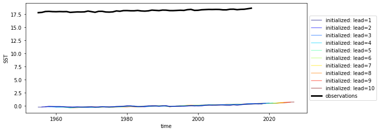
We have a huge bias because the initialized data is already converted to an anomaly, but uninitialized historical and observations is not.
[13]:
hindcast.remove_bias(alignment='same_verif').plot()
[13]:
<AxesSubplot:xlabel='time', ylabel='SST'>
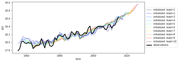
We still have a trend in all of our products, so we could also detrend them as well.
Detrend
Here we use a kitchen sink package called esmtools. It has a few vectorized stats functions that are dask-friendly.
We can leverage xarray’s .map() function to apply/map a function to all variables in our datasets.
[14]:
from esmtools.stats import rm_poly

hindcast_detrended = hindcast.map(rm_poly, order=2, dim='init').apply(rm_poly, order=2, dim='time')
hindcast_detrended.plot()
[14]:
<AxesSubplot:xlabel='time', ylabel='SST'>
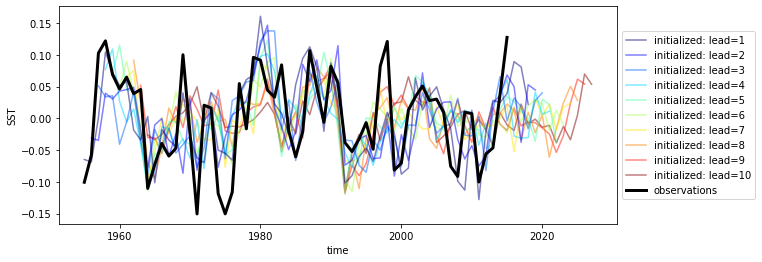
And it looks like everything got detrended by a quadratic fit! That wasn’t too hard.
Verify
Now that we’ve done our pre-processing, let’s quickly compute some metrics. Check the metrics page here for all the keywords you can use. The API is currently pretty simple for the HindcastEnsemble. You can essentially compute standard skill metrics and a reference persistence forecast.
[15]:
hindcast_detrended.verify(metric='mse',
                          comparison='e2o',
                          dim='init',
                          alignment='same_verif',
                          reference='persistence')
[15]:
<xarray.Dataset>
Dimensions: (lead: 10, skill: 2)
Coordinates:
* lead (lead) int32 1 2 3 4 5 6 7 8 9 10
* skill (skill) <U11 'initialized' 'persistence'
Data variables:
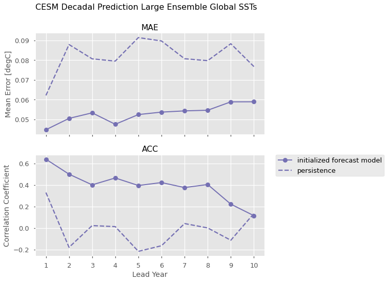
SST (skill, lead) float64 0.003274 0.004149 ... 0.01109 0.008786Here we leverage xarray’s plotting method to compute Mean Absolute Error and the Anomaly Correlation Coefficient against the ERSST observations, as well as the equivalent metrics computed for persistence forecasts for each of those metrics.
[16]:
import numpy as np

plt.style.use('ggplot')
plt.style.use('seaborn-talk')

color = '#7570b3'

f, axs = plt.subplots(nrows=2, figsize=(8, 8), sharex=True)

for ax, metric in zip(axs.ravel(), ['mae', 'acc']):
    handles = []
    result = hindcast_detrended.verify(metric=metric, comparison='e2o', dim='init',
                                 alignment='same_verif',reference='persistence')
    p1, = result.sel(skill='initialized').SST.plot(ax=ax,
                                       marker='o',
                                       color=color,
                                       label='initialized forecast model',
                                       linewidth=2)
    p2, = result.sel(skill='persistence').SST.plot(ax=ax,
                                             color=color,
                                             linestyle='--',
                                             label='persistence')
    handles.append(p1)
    handles.append(p2)
    ax.set_title(metric.upper())


axs[0].set_ylabel('Mean Error [degC]')
axs[1].set_ylabel('Correlation Coefficient')
axs[0].set_xlabel('')
axs[1].set_xlabel('Lead Year')
axs[1].set_xticks(np.arange(10)+1)

# matplotlib/xarray returning weirdness for the legend handles.
handles = [i.get_label() for i in handles]

# a little trick to put the legend on the outside.
plt.legend(handles, bbox_to_anchor=(1.05, 1), loc=2, borderaxespad=0.0)

plt.suptitle('CESM Decadal Prediction Large Ensemble Global SSTs', fontsize=16)
plt.show()
PerfectModelEnsemble
We’ll now play around a bit with the PerfectModelEnsemble object, using sample data from the MPI perfect model configuration.
[17]:
ds = load_dataset('MPI-PM-DP-1D') # initialized ensemble from MPI
control = load_dataset('MPI-control-1D') # base control run that initialized it

ds["lead"].attrs["units"] = "years"

print(ds)
<xarray.Dataset>
Dimensions:  (area: 3, init: 12, lead: 20, member: 10, period: 5)
Coordinates:
  * lead     (lead) int64 1 2 3 4 5 6 7 8 9 10 11 12 13 14 15 16 17 18 19 20
  * period   (period) object 'DJF' 'JJA' 'MAM' 'SON' 'ym'
  * area     (area) object 'global' 'North_Atlantic' 'North_Atlantic_SPG'
  * init     (init) int64 3014 3023 3045 3061 3124 ... 3175 3178 3228 3237 3257
  * member   (member) int64 0 1 2 3 4 5 6 7 8 9
Data variables:
    tos      (period, lead, area, init, member) float32 ...
    sos      (period, lead, area, init, member) float32 ...
    AMO      (period, lead, area, init, member) float32 ...
[18]:
pm = climpred.PerfectModelEnsemble(ds)
pm = pm.add_control(control)
print(pm)
<climpred.PerfectModelEnsemble>
Initialized Ensemble:
    tos      (period, lead, area, init, member) float32 ...
    sos      (period, lead, area, init, member) float32 ...
    AMO      (period, lead, area, init, member) float32 ...
Control:
    tos      (period, time, area) float32 ...
    sos      (period, time, area) float32 ...
    AMO      (period, time, area) float32 ...
Uninitialized:
    None
/Users/aaron.spring/Coding/climpred/climpred/utils.py:141: UserWarning: Assuming annual resolution due to numeric inits. Change init to a datetime if it is another resolution.
  "Assuming annual resolution due to numeric inits. "
Our objects are carrying sea surface temperature (tos), sea surface salinity (sos), and the Atlantic Multidecadal Oscillation index (AMO). Say we just want to look at skill metrics for temperature and salinity over the North Atlantic in JJA. We can just call a few easy xarray commands to filter down our object.
[19]:
pm = pm[['tos', 'sos']].sel(area='North_Atlantic', period='JJA')
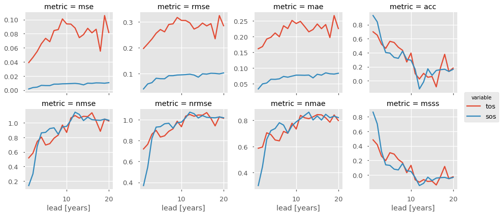
Now we can easily compute for a host of metrics. Here I just show a number of deterministic skill metrics comparing all individual members to the initialized ensemble mean. See comparisons for more information on the comparison keyword.
[20]:
METRICS = ['mse', 'rmse', 'mae', 'acc',
           'nmse', 'nrmse', 'nmae', 'msss']

result = []
for metric in METRICS:
    result.append(pm.verify(metric=metric, comparison='m2e', dim=['init','member']))

result = xr.concat(result, 'metric')
result['metric'] = METRICS

# Leverage the `xarray` plotting wrapper to plot all results at once.
result.to_array().plot(col='metric',
                       hue='variable',
                       col_wrap=4,
                       sharey=False,
                       sharex=True)
[20]:
<xarray.plot.facetgrid.FacetGrid at 0x7f95979b48d0>
It is useful to compare the initialized ensemble to an uninitialized run. See terminology for a description on “uninitialized” simulations. This gives us information about how initializations lead to enhanced predictability over knowledge of external forcing, whereas a comparison to persistence just tells us how well a dynamical forecast simulation does in comparison to a naive method. We can use the generate_uninitialized() method to bootstrap the control run and
create a pseudo-ensemble that approximates what an uninitialized ensemble would look like.
[21]:
pm = pm.generate_uninitialized()
pm
[21]:
<climpred.PerfectModelEnsemble>
Initialized Ensemble:
    tos      (lead, init, member) float32 13.464135 13.641711 ... 13.568891
    sos      (lead, init, member) float32 33.183903 33.146976 ... 33.25843
Control:
    tos      (time) float32 13.499312 13.742612 ... 13.076672 13.465583
    sos      (time) float32 33.232624 33.188156 33.201694 ... 33.16359 33.18352
Uninitialized:
    tos      (lead, init, member) float32 13.446274 13.426196 ... 13.7393265
    sos      (lead, init, member) float32 33.193344 33.200825 ... 33.359787
[22]:
pm = pm[['sos']] # Just assess for salinity.
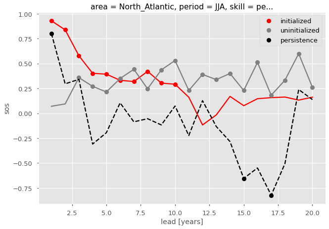
Here we plot the ACC for the initialized, uninitialized, and persistence forecasts for North Atlantic sea surface salinity in JJA. We add circles to the lines if the correlations are statistically significant for  .
.
[23]:
def plot_result(acc, pval, skill, color, label, linestyle='-'):
    """Helper function for cleaner plotting code."""
    acc.sel(skill=skill)['sos'].plot(color=color, linestyle=linestyle)
    masked_acc = acc.sel(skill=skill)['sos'].where(pval.sel(skill=skill)['sos'] <= 0.05)
    masked_acc.plot(marker='o', linestyle='None', color=color, label=label)

acc_result = pm.verify(metric='acc', comparison='m2e', dim=['init', 'member'] ,reference=['persistence', 'uninitialized'])
pval_result = pm.verify(metric='p_pval', comparison='m2e', dim=['init', 'member'], reference=['persistence', 'uninitialized'])

# ACC for initialized ensemble
plot_result(acc_result, pval_result, 'initialized', 'red', 'initialized')
plot_result(acc_result, pval_result, 'uninitialized', 'gray', 'uninitialized')
plot_result(acc_result, pval_result, 'persistence', 'black', 'persistence', linestyle='--')

plt.legend()
[23]:
<matplotlib.legend.Legend at 0x7f95968f81d0>
[ ]: