Calculate Seasonal ENSO Skill¶

In this example, we demonstrate:¶

How to remotely access data from the North American Multi-model Ensemble (NMME) hindcast database and set it up to be used in climpred
How to calculate the Anomaly Correlation Coefficient (ACC) using seasonal data

The North American Multi-model Ensemble (NMME)¶

Further information on NMME is available from Kirtman et al. 2014 and the NMME project website

The NMME public database is hosted on the International Research Institute for Climate and Society (IRI) data server http://iridl.ldeo.columbia.edu/SOURCES/.Models/.NMME/

Definitions¶

Anomalies: Departure from normal, where normal is defined as the climatological value based on the average value for each month over all years.
Nino3.4: An index used to represent the evolution of the El Nino-Southern Oscillation (ENSO). Calculated as the average sea surface temperature (SST) anomalies in the region 5S-5N; 190-240

[1]:

import warnings

import matplotlib.pyplot as plt
import xarray as xr
import pandas as pd
import numpy as np

from climpred import HindcastEnsemble
import climpred

[2]:

warnings.filterwarnings("ignore")

[3]:

def decode_cf(ds, time_var):
    if ds[time_var].attrs['calendar'] == '360':
        ds[time_var].attrs['calendar'] = '360_day'
    ds = xr.decode_cf(ds, decode_times=True)
    return ds

Load the monthly sea surface temperature (SST) hindcast data for the NCEP-CFSv2 model from the data server

[4]:

# Get NMME data for NCEP-CFSv2, SST
url = 'http://iridl.ldeo.columbia.edu/SOURCES/.Models/.NMME/NCEP-CFSv2/.HINDCAST/.MONTHLY/.sst/dods'
fcstds = decode_cf(xr.open_dataset(url, decode_times=False, chunks={'S': 1, 'L': 12}), 'S')
fcstds

[4]:

<xarray.Dataset>
Dimensions:  (L: 10, M: 24, S: 348, X: 360, Y: 181)
Coordinates:
  * S        (S) object 1982-01-01 00:00:00 ... 2010-12-01 00:00:00
  * M        (M) float32 1.0 2.0 3.0 4.0 5.0 6.0 ... 20.0 21.0 22.0 23.0 24.0
  * X        (X) float32 0.0 1.0 2.0 3.0 4.0 ... 355.0 356.0 357.0 358.0 359.0
  * L        (L) float32 0.5 1.5 2.5 3.5 4.5 5.5 6.5 7.5 8.5 9.5
  * Y        (Y) float32 -90.0 -89.0 -88.0 -87.0 -86.0 ... 87.0 88.0 89.0 90.0
Data variables:
    sst      (S, L, M, Y, X) float32 dask.array<chunksize=(1, 10, 24, 181, 360), meta=np.ndarray>
Attributes:
    Conventions:  IRIDL

The NMME data dimensions correspond to the following climpred dimension definitions: X=lon,L=lead,Y=lat,M=member, S=init. We will rename the dimensions to their climpred names.

[5]:

fcstds=fcstds.rename({'S': 'init','L': 'lead','M': 'member', 'X': 'lon', 'Y': 'lat'})

Let’s make sure that the lead dimension is set properly for climpred. NMME data stores leads as 0.5, 1.5, 2.5, etc, which correspond to 0, 1, 2, … months since initialization. We will change the lead to be integers starting with zero.

[6]:

fcstds['lead']=(fcstds['lead']-0.5).astype('int')

Now we need to make sure that the init dimension is set properly for climpred. For monthly data, the init dimension must be a xr.cfdateTimeIndex or a pd.datetimeIndex. We convert the init values to pd.datatimeIndex.

[7]:

fcstds['init']=pd.to_datetime(fcstds.init.values.astype(str))
fcstds['init']=pd.to_datetime(fcstds['init'].dt.strftime('%Y%m01 00:00'))

Next, we want to get the verification SST data from the data server

[8]:

obsurl='http://iridl.ldeo.columbia.edu/SOURCES/.Models/.NMME/.OIv2_SST/.sst/dods'
verifds = decode_cf(xr.open_dataset(obsurl, decode_times=False),'T')
verifds

[8]:

<xarray.Dataset>
Dimensions:  (T: 405, X: 360, Y: 181)
Coordinates:
  * Y        (Y) float32 -90.0 -89.0 -88.0 -87.0 -86.0 ... 87.0 88.0 89.0 90.0
  * X        (X) float32 0.0 1.0 2.0 3.0 4.0 ... 355.0 356.0 357.0 358.0 359.0
  * T        (T) object 1982-01-16 00:00:00 ... 2015-09-16 00:00:00
Data variables:
    sst      (T, Y, X) float32 ...
Attributes:
    Conventions:  IRIDL

Rename the dimensions to correspond to climpred dimensions

[9]:

verifds=verifds.rename({'T': 'time','X': 'lon', 'Y': 'lat'})

Convert the time data to be of type pd.datetimeIndex

[10]:

verifds['time']=pd.to_datetime(verifds.time.values.astype(str))
verifds['time']=pd.to_datetime(verifds['time'].dt.strftime('%Y%m01 00:00'))
verifds

[10]:

<xarray.Dataset>
Dimensions:  (lat: 181, lon: 360, time: 405)
Coordinates:
  * lat      (lat) float32 -90.0 -89.0 -88.0 -87.0 -86.0 ... 87.0 88.0 89.0 90.0
  * lon      (lon) float32 0.0 1.0 2.0 3.0 4.0 ... 355.0 356.0 357.0 358.0 359.0
  * time     (time) datetime64[ns] 1982-01-01 1982-02-01 ... 2015-09-01
Data variables:
    sst      (time, lat, lon) float32 ...
Attributes:
    Conventions:  IRIDL

Subset the data to 1982-2010

[11]:

verifds=verifds.sel(time=slice('1982-01-01','2010-12-01'))
fcstds=fcstds.sel(init=slice('1982-01-01','2010-12-01'))

Calculate the Nino3.4 index for forecast and verification

[12]:

fcstnino34=fcstds.sel(lat=slice(-5,5),lon=slice(190,240)).mean(['lat','lon'])
verifnino34=verifds.sel(lat=slice(-5,5),lon=slice(190,240)).mean(['lat','lon'])

fcstclimo = fcstnino34.groupby('init.month').mean('init')
fcstanoms = (fcstnino34.groupby('init.month') - fcstclimo)

verifclimo = verifnino34.groupby('time.month').mean('time')
verifanoms = (verifnino34.groupby('time.month') - verifclimo)

print(fcstanoms)
print(verifanoms)

<xarray.Dataset>
Dimensions:  (init: 348, lead: 10, member: 24)
Coordinates:
  * lead     (lead) int64 0 1 2 3 4 5 6 7 8 9
  * member   (member) float32 1.0 2.0 3.0 4.0 5.0 ... 20.0 21.0 22.0 23.0 24.0
  * init     (init) datetime64[ns] 1982-01-01 1982-02-01 ... 2010-12-01
    month    (init) int64 1 2 3 4 5 6 7 8 9 10 11 ... 2 3 4 5 6 7 8 9 10 11 12
Data variables:
    sst      (init, lead, member) float32 dask.array<chunksize=(1, 10, 24), meta=np.ndarray>
<xarray.Dataset>
Dimensions:  (time: 348)
Coordinates:
  * time     (time) datetime64[ns] 1982-01-01 1982-02-01 ... 2010-12-01
    month    (time) int64 1 2 3 4 5 6 7 8 9 10 11 ... 2 3 4 5 6 7 8 9 10 11 12
Data variables:
    sst      (time) float32 0.14492226 -0.044160843 ... -1.5685654 -1.6083965

Make Seasonal Averages with center=True and drop NaNs. This means that the first value

[13]:

fcstnino34seas=fcstanoms.rolling(lead=3, center=True).mean().dropna(dim='lead')
verifnino34seas=verifanoms.rolling(time=3, center=True).mean().dropna(dim='time')

Create new xr.DataArray with seasonal data

[14]:

nleads=fcstnino34seas['lead'][::3].size
fcst=xr.DataArray(fcstnino34seas['sst'][:,::3,:],
                           coords={'init' : fcstnino34seas['init'],
                                   'lead': np.arange(0,nleads),
                                   'member': fcstanoms['member'],
                                   },
                           dims=['init','lead','member'])
fcst.name = 'sst'

Assign the units attribute of seasons to the lead dimension

[15]:

fcst['lead'].attrs={'units': 'seasons'}

Create a climpred HindcastEnsemble object

[16]:

hindcast = HindcastEnsemble(fcst)
hindcast = hindcast.add_observations(verifnino34seas, 'observations')

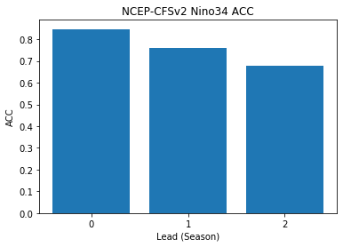
Compute the Anomaly Correlation Coefficient (ACC) 0, 1, 2, and 3 season lead-times

[17]:

skillds = hindcast.verify(metric='acc')
print(skillds)

<xarray.Dataset>
Dimensions:  (lead: 3)
Coordinates:
  * lead     (lead) int64 0 1 2
Data variables:
    sst      (lead) float64 0.847 0.7614 0.6779
Attributes:
    prediction_skill:              calculated by climpred https://climpred.re...
    skill_calculated_by_function:  compute_hindcast
    number_of_initializations:     348
    number_of_members:             24
    metric:                        pearson_r
    comparison:                    e2o
    dim:                           time
    units:                         None
    created:                       2020-01-21 11:41:35

Make bar plot of Nino3.4 skill for 0,1, and 2 season lead times

[18]:

x=np.arange(0,nleads,1.0).astype(int)
plt.bar(x,skillds['sst'])
plt.xticks(x)
plt.title('NCEP-CFSv2 Nino34 ACC')
plt.xlabel('Lead (Season)')
plt.ylabel('ACC')

[18]:

Text(0, 0.5, 'ACC')

../../_images/examples_monseas_seasonal-enso-subx-example_36_1.png

References¶

Kirtman, B.P., D. Min, J.M. Infanti, J.L. Kinter, D.A. Paolino, Q. Zhang, H. van den Dool, S. Saha, M.P. Mendez, E. Becker, P. Peng, P. Tripp, J. Huang, D.G. DeWitt, M.K. Tippett, A.G. Barnston, S. Li, A. Rosati, S.D. Schubert, M. Rienecker, M. Suarez, Z.E. Li, J. Marshak, Y. Lim, J. Tribbia, K. Pegion, W.J. Merryfield, B. Denis, and E.F. Wood, 2014: The North American Multimodel Ensemble: Phase-1 Seasonal-to-Interannual Prediction; Phase-2 toward Developing Intraseasonal Prediction. Bull. Amer. Meteor. Soc., 95, 585–601, https://doi.org/10.1175/BAMS-D-12-00050.1