Metrics
All high-level functions have an optional metric argument that can be called to
determine which metric is used in computing predictability.
Note
We use the phrase ‘observations’ o here to refer to the ‘truth’ data to which
we compare the forecast f. These metrics can also be applied relative
to a control simulation, reconstruction, observations, etc. This would just
change the resulting score from quantifying skill to quantifying potential
predictability.
Internally, all metric functions require forecast and observations as inputs.
The dimension dim is set internally by
compute_hindcast() or
compute_perfect_model() to specify over which dimensions
the metric is applied. See Comparisons for more on the dim argument.
Deterministic
Deterministic metrics assess the forecast as a definite prediction of the future, rather than in terms of probabilities. Another way to look at deterministic metrics is that they are a special case of probabilistic metrics where a value of one is assigned to one category and zero to all others [Jolliffe2011].
Correlation Metrics
The below metrics rely fundamentally on correlations in their computation. In the
literature, correlation metrics are typically referred to as the Anomaly Correlation
Coefficient (ACC). This implies that anomalies in the forecast and observations
are being correlated. Typically, this is computed using the linear
Pearson Product-Moment Correlation.
However, climpred also offers the
Spearman’s Rank Correlation.
Note that the p value associated with these correlations is computed via a separate
metric. Use pearson_r_p_value or spearman_r_p_value to compute p values assuming
that all samples in the correlated time series are independent. Use
pearson_r_eff_p_value or spearman_r_eff_p_value to account for autocorrelation
in the time series by calculating the effective_sample_size.
Pearson Product-Moment Correlation Coefficient
# Enter any of the below keywords in ``metric=...`` for the compute functions.
In [1]: print(f"\n\nKeywords: {metric_aliases['pearson_r']}")


Keywords: ['pearson_r', 'pr', 'acc', 'pacc']
-
climpred.metrics._pearson_r(forecast, verif, dim=None, **metric_kwargs)[source]¶ Pearson product-moment correlation coefficient.
A measure of the linear association between the forecast and verification data that is independent of the mean and variance of the individual distributions. This is also known as the Anomaly Correlation Coefficient (ACC) when correlating anomalies.
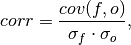
where
 and
and  represent the standard deviation
of the forecast and verification data over the experimental period, respectively.
represent the standard deviation
of the forecast and verification data over the experimental period, respectively.Note
Use metric
pearson_r_p_valueorpearson_r_eff_p_valueto get the corresponding p value.Parameters: - forecast (xarray object) – Forecast.
- verif (xarray object) – Verification data.
- dim (str) – Dimension(s) to perform metric over. Automatically set by compute function.
- weights (xarray object, optional) – Weights to apply over dimension. Defaults to
None. - skipna (bool, optional) – If True, skip NaNs over dimension being applied to.
Defaults to
False.
- Details:
minimum -1.0 maximum 1.0 perfect 1.0 orientation positive
See also
- xskillscore.pearson_r
- xskillscore.pearson_r_p_value
- climpred.pearson_r_p_value
- climpred.pearson_r_eff_p_value
Pearson Correlation p value
# Enter any of the below keywords in ``metric=...`` for the compute functions.
In [2]: print(f"\n\nKeywords: {metric_aliases['pearson_r_p_value']}")


Keywords: ['pearson_r_p_value', 'p_pval', 'pvalue', 'pval']
-
climpred.metrics._pearson_r_p_value(forecast, verif, dim=None, **metric_kwargs)[source]¶ Probability that forecast and verification data are linearly uncorrelated.
Two-tailed p value associated with the Pearson product-moment correlation coefficient (
pearson_r), assuming that all samples are independent. Usepearson_r_eff_p_valueto account for autocorrelation in the forecast and verification data.Parameters: - forecast (xarray object) – Forecast.
- verif (xarray object) – Verification data.
- dim (str) – Dimension(s) to perform metric over. Automatically set by compute function.
- weights (xarray object, optional) – Weights to apply over dimension. Defaults to
None. - skipna (bool, optional) – If True, skip NaNs over dimension being applied to.
Defaults to
False.
- Details:
minimum 0.0 maximum 1.0 perfect 1.0 orientation negative
See also
- xskillscore.pearson_r
- xskillscore.pearson_r_p_value
- climpred.pearson_r
- climpred.pearson_r_eff_p_value
Effective Sample Size
# Enter any of the below keywords in ``metric=...`` for the compute functions.
In [3]: print(f"\n\nKeywords: {metric_aliases['effective_sample_size']}")


Keywords: ['effective_sample_size', 'n_eff', 'eff_n']
-
climpred.metrics._effective_sample_size(forecast, verif, dim=None, **metric_kwargs)[source]¶ Effective sample size for temporally correlated data.
Note
Weights are not included here due to the dependence on temporal autocorrelation.
Note
This metric can only be used for hindcast-type simulations.
The effective sample size extracts the number of independent samples between two time series being correlated. This is derived by assessing the magnitude of the lag-1 autocorrelation coefficient in each of the time series being correlated. A higher autocorrelation induces a lower effective sample size which raises the correlation coefficient for a given p value.
The effective sample size is used in computing the effective p value. See
pearson_r_eff_p_valueandspearman_r_eff_p_value.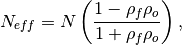
where
 and
and  are the lag-1 autocorrelation
coefficients for the forecast and verification data.
are the lag-1 autocorrelation
coefficients for the forecast and verification data.Parameters: - forecast (xarray object) – Forecast.
- verif (xarray object) – Verification data.
- dim (str) – Dimension(s) to perform metric over. Automatically set by compute function.
- skipna (bool, optional) – If True, skip NaNs over dimension being applied to.
Defaults to
False.
- Details:
minimum 0.0 maximum ∞ perfect N/A orientation positive - Reference:
- Bretherton, Christopher S., et al. “The effective number of spatial degrees of freedom of a time-varying field.” Journal of climate 12.7 (1999): 1990-2009.
Pearson Correlation Effective p value
# Enter any of the below keywords in ``metric=...`` for the compute functions.
In [4]: print(f"\n\nKeywords: {metric_aliases['pearson_r_eff_p_value']}")


Keywords: ['pearson_r_eff_p_value', 'p_pval_eff', 'pvalue_eff', 'pval_eff']
-
climpred.metrics._pearson_r_eff_p_value(forecast, verif, dim=None, **metric_kwargs)[source]¶ Probability that forecast and verification data are linearly uncorrelated, accounting for autocorrelation.
Note
Weights are not included here due to the dependence on temporal autocorrelation.
Note
This metric can only be used for hindcast-type simulations.
The effective p value is computed by replacing the sample size
 in the
t-statistic with the effective sample size,
in the
t-statistic with the effective sample size,  . The same Pearson
product-moment correlation coefficient
. The same Pearson
product-moment correlation coefficient  is used as when computing the
standard p value.
is used as when computing the
standard p value.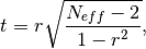
where
is computed via the autocorrelation in the forecast and
verification data.where
and are the lag-1 autocorrelation
coefficients for the forecast and verification data.Parameters: - forecast (xarray object) – Forecast.
- verif (xarray object) – Verification data.
- dim (str) – Dimension(s) to perform metric over. Automatically set by compute function.
- skipna (bool, optional) – If True, skip NaNs over dimension being applied to.
Defaults to
False.
- Details:
minimum 0.0 maximum 1.0 perfect 1.0 orientation negative
See also
- climpred.effective_sample_size
- climpred.spearman_r_eff_p_value
- Reference:
- Bretherton, Christopher S., et al. “The effective number of spatial degrees of freedom of a time-varying field.” Journal of climate 12.7 (1999): 1990-2009.
Spearman’s Rank Correlation Coefficient
# Enter any of the below keywords in ``metric=...`` for the compute functions.
In [5]: print(f"\n\nKeywords: {metric_aliases['spearman_r']}")


Keywords: ['spearman_r', 'sacc', 'sr']
-
climpred.metrics._spearman_r(forecast, verif, dim=None, **metric_kwargs)[source]¶ Spearman’s rank correlation coefficient.

This correlation coefficient is nonparametric and assesses how well the relationship between the forecast and verification data can be described using a monotonic function. It is computed by first ranking the forecasts and verification data, and then correlating those ranks using the
pearson_rcorrelation.This is also known as the anomaly correlation coefficient (ACC) when comparing anomalies, although the Pearson product-moment correlation coefficient (
pearson_r) is typically used when computing the ACC.Note
Use metric
spearman_r_p_valueorspearman_r_eff_p_valueto get the corresponding p value.Parameters: - forecast (xarray object) – Forecast.
- verif (xarray object) – Verification data.
- dim (str) – Dimension(s) to perform metric over. Automatically set by compute function.
- weights (xarray object, optional) – Weights to apply over dimension. Defaults to
None. - skipna (bool, optional) – If True, skip NaNs over dimension being applied to.
Defaults to
False.
- Details:
minimum -1.0 maximum 1.0 perfect 1.0 orientation positive
See also
- xskillscore.spearman_r
- xskillscore.spearman_r_p_value
- climpred.spearman_r_p_value
- climpred.spearman_r_eff_p_value
Spearman’s Rank Correlation Coefficient p value
# Enter any of the below keywords in ``metric=...`` for the compute functions.
In [6]: print(f"\n\nKeywords: {metric_aliases['spearman_r_p_value']}")


Keywords: ['spearman_r_p_value', 's_pval', 'spvalue', 'spval']
-
climpred.metrics._spearman_r_p_value(forecast, verif, dim=None, **metric_kwargs)[source]¶ Probability that forecast and verification data are monotonically uncorrelated.
Two-tailed p value associated with the Spearman’s rank correlation coefficient (
spearman_r), assuming that all samples are independent. Usespearman_r_eff_p_valueto account for autocorrelation in the forecast and verification data.Parameters: - forecast (xarray object) – Forecast.
- verif (xarray object) – Verification data.
- dim (str) – Dimension(s) to perform metric over. Automatically set by compute function.
- weights (xarray object, optional) – Weights to apply over dimension. Defaults to
None. - skipna (bool, optional) – If True, skip NaNs over dimension being applied to.
Defaults to
False.
- Details:
minimum 0.0 maximum 1.0 perfect 1.0 orientation negative
See also
- xskillscore.spearman_r
- xskillscore.spearman_r_p_value
- climpred.spearman_r
- climpred.spearman_r_eff_p_value
Spearman’s Rank Correlation Effective p value
# Enter any of the below keywords in ``metric=...`` for the compute functions.
In [7]: print(f"\n\nKeywords: {metric_aliases['spearman_r_eff_p_value']}")


Keywords: ['spearman_r_eff_p_value', 's_pval_eff', 'spvalue_eff', 'spval_eff']
-
climpred.metrics._spearman_r_eff_p_value(forecast, verif, dim=None, **metric_kwargs)[source]¶ Probability that forecast and verification data are monotonically uncorrelated, accounting for autocorrelation.
Note
Weights are not included here due to the dependence on temporal autocorrelation.
Note
This metric can only be used for hindcast-type simulations.
The effective p value is computed by replacing the sample size
in the
t-statistic with the effective sample size, . The same Spearman’s
rank correlation coefficient is used as when computing the standard p
value.where
is computed via the autocorrelation in the forecast and
verification data.where
and are the lag-1 autocorrelation
coefficients for the forecast and verification data.Parameters: - forecast (xarray object) – Forecast.
- verif (xarray object) – Verification data.
- dim (str) – Dimension(s) to perform metric over. Automatically set by compute function.
- skipna (bool, optional) – If True, skip NaNs over dimension being applied to.
Defaults to
False.
- Details:
minimum 0.0 maximum 1.0 perfect 1.0 orientation negative
See also
- climpred.effective_sample_size
- climpred.pearson_r_eff_p_value
- Reference:
- Bretherton, Christopher S., et al. “The effective number of spatial degrees of freedom of a time-varying field.” Journal of climate 12.7 (1999): 1990-2009.
Distance Metrics
This class of metrics simply measures the distance (or difference) between forecasted values and observed values.
Mean Squared Error (MSE)
# Enter any of the below keywords in ``metric=...`` for the compute functions.
In [8]: print(f"\n\nKeywords: {metric_aliases['mse']}")


Keywords: ['mse']
-
climpred.metrics._mse(forecast, verif, dim=None, **metric_kwargs)[source]¶ Mean Sqaure Error (MSE).
The average of the squared difference between forecasts and verification data. This incorporates both the variance and bias of the estimator. Because the error is squared, it is more sensitive to large forecast errors than
mae, and thus a more conservative metric. For example, a single error of 2°C counts the same as two 1°C errors when usingmae. On the other hand, the 2°C error counts double formse. See Jolliffe and Stephenson, 2011.Parameters: - forecast (xarray object) – Forecast.
- verif (xarray object) – Verification data.
- dim (str) – Dimension(s) to perform metric over. Automatically set by compute function.
- weights (xarray object, optional) – Weights to apply over dimension. Defaults to
None. - skipna (bool, optional) – If True, skip NaNs over dimension being applied to.
Defaults to
False.
- Details:
minimum 0.0 maximum ∞ perfect 0.0 orientation negative
See also
- xskillscore.mse
- Reference:
- Ian T. Jolliffe and David B. Stephenson. Forecast Verification: A Practitioner’s Guide in Atmospheric Science. John Wiley & Sons, Ltd, Chichester, UK, December 2011. ISBN 978-1-119-96000-3 978-0-470-66071-3. URL: http://doi.wiley.com/10.1002/9781119960003.
Root Mean Square Error (RMSE)
# Enter any of the below keywords in ``metric=...`` for the compute functions.
In [9]: print(f"\n\nKeywords: {metric_aliases['rmse']}")


Keywords: ['rmse']
-
climpred.metrics._rmse(forecast, verif, dim=None, **metric_kwargs)[source]¶ Root Mean Sqaure Error (RMSE).
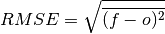
The square root of the average of the squared differences between forecasts and verification data.
Parameters: - forecast (xarray object) – Forecast.
- verif (xarray object) – Verification data.
- dim (str) – Dimension(s) to perform metric over. Automatically set by compute function.
- weights (xarray object, optional) – Weights to apply over dimension. Defaults to
None. - skipna (bool, optional) – If True, skip NaNs over dimension being applied to.
Defaults to
False.
- Details:
minimum 0.0 maximum ∞ perfect 0.0 orientation negative
See also
- xskillscore.rmse
Mean Absolute Error (MAE)
# Enter any of the below keywords in ``metric=...`` for the compute functions.
In [10]: print(f"\n\nKeywords: {metric_aliases['mae']}")


Keywords: ['mae']
-
climpred.metrics._mae(forecast, verif, dim=None, **metric_kwargs)[source]¶ Mean Absolute Error (MAE).
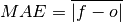
The average of the absolute differences between forecasts and verification data. A more robust measure of forecast accuracy than
msewhich is sensitive to large outlier forecast errors.Parameters: - forecast (xarray object) – Forecast.
- verif (xarray object) – Verification data.
- dim (str) – Dimension(s) to perform metric over. Automatically set by compute function.
- weights (xarray object, optional) – Weights to apply over dimension. Defaults to
None. - skipna (bool, optional) – If True, skip NaNs over dimension being applied to.
Defaults to
False.
- Details:
minimum 0.0 maximum ∞ perfect 0.0 orientation negative
See also
- xskillscore.mae
- Reference:
- Ian T. Jolliffe and David B. Stephenson. Forecast Verification: A Practitioner’s Guide in Atmospheric Science. John Wiley & Sons, Ltd, Chichester, UK, December 2011. ISBN 978-1-119-96000-3 978-0-470-66071-3. URL: http://doi.wiley.com/10.1002/9781119960003.
Median Absolute Error
# Enter any of the below keywords in ``metric=...`` for the compute functions.
In [11]: print(f"\n\nKeywords: {metric_aliases['median_absolute_error']}")


Keywords: ['median_absolute_error']
-
climpred.metrics._median_absolute_error(forecast, verif, dim=None, **metric_kwargs)[source]¶ Median Absolute Error.
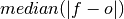
The median of the absolute differences between forecasts and verification data. Applying the median function to absolute error makes it more robust to outliers.
Parameters: - forecast (xarray object) – Forecast.
- verif (xarray object) – Verification data.
- dim (str) – Dimension(s) to perform metric over. Automatically set by compute function.
- skipna (bool, optional) – If True, skip NaNs over dimension being applied to.
Defaults to
False.
- Details:
minimum 0.0 maximum ∞ perfect 0.0 orientation negative
See also
- xskillscore.median_absolute_error
Normalized Distance Metrics
Distance metrics like mse can be normalized to 1. The normalization factor
depends on the comparison type choosen. For example, the distance between an ensemble
member and the ensemble mean is half the distance of an ensemble member with other
ensemble members. See _get_norm_factor().
Normalized Mean Square Error (NMSE)
# Enter any of the below keywords in ``metric=...`` for the compute functions.
In [12]: print(f"\n\nKeywords: {metric_aliases['nmse']}")


Keywords: ['nmse', 'nev']
-
climpred.metrics._nmse(forecast, verif, dim=None, **metric_kwargs)[source]¶ Normalized MSE (NMSE), also known as Normalized Ensemble Variance (NEV).
Mean Square Error (
mse) normalized by the variance of the verification data.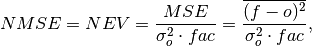
where
 is 1 when using comparisons involving the ensemble mean (
m2e,e2c,e2o) and 2 when using comparisons involving individual ensemble members (m2c,m2m,m2o). See_get_norm_factor().Note
climpreduses a single-valued internal reference forecast for the NMSE, in the terminology of Murphy 1988. I.e., we use a single climatological variance of the verification data within the experimental window for normalizing MSE.Parameters: - forecast (xarray object) – Forecast.
- verif (xarray object) – Verification data.
- dim (str) – Dimension(s) to perform metric over. Automatically set by compute function.
- weights (xarray object, optional) – Weights to apply over dimension. Defaults to
None. - skipna (bool, optional) – If True, skip NaNs over dimension being applied to.
Defaults to
False. - comparison (str) – Name comparison needed for normalization factor fac, see
_get_norm_factor()(Handled internally by the compute functions)
- Details:
minimum 0.0 maximum ∞ perfect 0.0 orientation negative better than climatology 0.0 - 1.0 worse than climatology > 1.0 - Reference:
- Griffies, S. M., and K. Bryan. “A Predictability Study of Simulated North Atlantic Multidecadal Variability.” Climate Dynamics 13, no. 7–8 (August 1, 1997): 459–87. https://doi.org/10/ch4kc4.
- Murphy, Allan H. “Skill Scores Based on the Mean Square Error and Their Relationships to the Correlation Coefficient.” Monthly Weather Review 116, no. 12 (December 1, 1988): 2417–24. https://doi.org/10/fc7mxd.
Normalized Mean Absolute Error (NMAE)
# Enter any of the below keywords in ``metric=...`` for the compute functions.
In [13]: print(f"\n\nKeywords: {metric_aliases['nmae']}")


Keywords: ['nmae']
-
climpred.metrics._nmae(forecast, verif, dim=None, **metric_kwargs)[source]¶ Normalized Mean Absolute Error (NMAE).
Mean Absolute Error (
mae) normalized by the standard deviation of the verification data.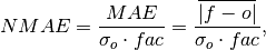
where
is 1 when using comparisons involving the ensemble mean (m2e,e2c,e2o) and 2 when using comparisons involving individual ensemble members (m2c,m2m,m2o). See_get_norm_factor().Note
climpreduses a single-valued internal reference forecast for the NMAE, in the terminology of Murphy 1988. I.e., we use a single climatological standard deviation of the verification data within the experimental window for normalizing MAE.Parameters: - forecast (xarray object) – Forecast.
- verif (xarray object) – Verification data.
- dim (str) – Dimension(s) to perform metric over. Automatically set by compute function.
- weights (xarray object, optional) – Weights to apply over dimension. Defaults to
None. - skipna (bool, optional) – If True, skip NaNs over dimension being applied to.
Defaults to
False. - comparison (str) – Name comparison needed for normalization factor fac, see
_get_norm_factor()(Handled internally by the compute functions)
- Details:
minimum 0.0 maximum ∞ perfect 0.0 orientation negative better than climatology 0.0 - 1.0 worse than climatology > 1.0 - Reference:
- Griffies, S. M., and K. Bryan. “A Predictability Study of Simulated North Atlantic Multidecadal Variability.” Climate Dynamics 13, no. 7–8 (August 1, 1997): 459–87. https://doi.org/10/ch4kc4.
- Murphy, Allan H. “Skill Scores Based on the Mean Square Error and Their Relationships to the Correlation Coefficient.” Monthly Weather Review 116, no. 12 (December 1, 1988): 2417–24. https://doi.org/10/fc7mxd.
Normalized Root Mean Square Error (NRMSE)
# Enter any of the below keywords in ``metric=...`` for the compute functions.
In [14]: print(f"\n\nKeywords: {metric_aliases['nrmse']}")


Keywords: ['nrmse']
-
climpred.metrics._nrmse(forecast, verif, dim=None, **metric_kwargs)[source]¶ Normalized Root Mean Square Error (NRMSE).
Root Mean Square Error (
rmse) normalized by the standard deviation of the verification data.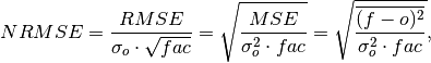
where
is 1 when using comparisons involving the ensemble mean (m2e,e2c,e2o) and 2 when using comparisons involving individual ensemble members (m2c,m2m,m2o). See_get_norm_factor().Note
climpreduses a single-valued internal reference forecast for the NRMSE, in the terminology of Murphy 1988. I.e., we use a single climatological variance of the verification data within the experimental window for normalizing RMSE.Parameters: - forecast (xarray object) – Forecast.
- verif (xarray object) – Verification data.
- dim (str) – Dimension(s) to perform metric over. Automatically set by compute function.
- weights (xarray object, optional) – Weights to apply over dimension. Defaults to
None. - skipna (bool, optional) – If True, skip NaNs over dimension being applied to.
Defaults to
False. - comparison (str) – Name comparison needed for normalization factor fac, see
_get_norm_factor()(Handled internally by the compute functions)
- Details:
minimum 0.0 maximum ∞ perfect 0.0 orientation negative better than climatology 0.0 - 1.0 worse than climatology > 1.0 - Reference:
- Bushuk, Mitchell, Rym Msadek, Michael Winton, Gabriel Vecchi, Xiaosong Yang, Anthony Rosati, and Rich Gudgel. “Regional Arctic Sea–Ice Prediction: Potential versus Operational Seasonal Forecast Skill.” Climate Dynamics, June 9, 2018. https://doi.org/10/gd7hfq.
- Hawkins, Ed, Steffen Tietsche, Jonathan J. Day, Nathanael Melia, Keith Haines, and Sarah Keeley. “Aspects of Designing and Evaluating Seasonal-to-Interannual Arctic Sea-Ice Prediction Systems.” Quarterly Journal of the Royal Meteorological Society 142, no. 695 (January 1, 2016): 672–83. https://doi.org/10/gfb3pn.
- Murphy, Allan H. “Skill Scores Based on the Mean Square Error and Their Relationships to the Correlation Coefficient.” Monthly Weather Review 116, no. 12 (December 1, 1988): 2417–24. https://doi.org/10/fc7mxd.
Mean Square Error Skill Score (MSESS)
# Enter any of the below keywords in ``metric=...`` for the compute functions.
In [15]: print(f"\n\nKeywords: {metric_aliases['msess']}")


Keywords: ['msess', 'ppp', 'msss']
-
climpred.metrics._msess(forecast, verif, dim=None, **metric_kwargs)[source]¶ Mean Squared Error Skill Score (MSESS).
where
is 1 when using comparisons involving the ensemble mean (m2e,e2c,e2o) and 2 when using comparisons involving individual ensemble members (m2c,m2m,m2o). See_get_norm_factor().This skill score can be intepreted as a percentage improvement in accuracy. I.e., it can be multiplied by 100%.
Note
climpreduses a single-valued internal reference forecast for the MSSS, in the terminology of Murphy 1988. I.e., we use a single climatological variance of the verification data within the experimental window for normalizing MSE.Parameters: - forecast (xarray object) – Forecast.
- verif (xarray object) – Verification data.
- dim (str) – Dimension(s) to perform metric over. Automatically set by compute function.
- weights (xarray object, optional) – Weights to apply over dimension. Defaults to
None. - skipna (bool, optional) – If True, skip NaNs over dimension being applied to.
Defaults to
False. - comparison (str) – Name comparison needed for normalization factor fac, see
_get_norm_factor()(Handled internally by the compute functions)
- Details:
minimum -∞ maximum 1.0 perfect 1.0 orientation positive better than climatology > 0.0 equal to climatology 0.0 worse than climatology < 0.0 - Reference:
- Griffies, S. M., and K. Bryan. “A Predictability Study of Simulated North Atlantic Multidecadal Variability.” Climate Dynamics 13, no. 7–8 (August 1, 1997): 459–87. https://doi.org/10/ch4kc4.
- Murphy, Allan H. “Skill Scores Based on the Mean Square Error and Their Relationships to the Correlation Coefficient.” Monthly Weather Review 116, no. 12 (December 1, 1988): 2417–24. https://doi.org/10/fc7mxd.
- Pohlmann, Holger, Michael Botzet, Mojib Latif, Andreas Roesch, Martin Wild, and Peter Tschuck. “Estimating the Decadal Predictability of a Coupled AOGCM.” Journal of Climate 17, no. 22 (November 1, 2004): 4463–72. https://doi.org/10/d2qf62.
- Bushuk, Mitchell, Rym Msadek, Michael Winton, Gabriel Vecchi, Xiaosong Yang, Anthony Rosati, and Rich Gudgel. “Regional Arctic Sea–Ice Prediction: Potential versus Operational Seasonal Forecast Skill. Climate Dynamics, June 9, 2018. https://doi.org/10/gd7hfq.
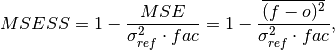
Mean Absolute Percentage Error (MAPE)
# Enter any of the below keywords in ``metric=...`` for the compute functions.
In [16]: print(f"\n\nKeywords: {metric_aliases['mape']}")


Keywords: ['mape']
-
climpred.metrics._mape(forecast, verif, dim=None, **metric_kwargs)[source]¶ Mean Absolute Percentage Error (MAPE).
Mean absolute error (
mae) expressed as the fractional error relative to the verification data.
Parameters: - forecast (xarray object) – Forecast.
- verif (xarray object) – Verification data.
- dim (str) – Dimension(s) to perform metric over. Automatically set by compute function.
- weights (xarray object, optional) – Weights to apply over dimension. Defaults to
None. - skipna (bool, optional) – If True, skip NaNs over dimension being applied to.
Defaults to
False.
- Details:
minimum 0.0 maximum ∞ perfect 0.0 orientation negative
See also
- xskillscore.mape
Symmetric Mean Absolute Percentage Error (sMAPE)
# Enter any of the below keywords in ``metric=...`` for the compute functions.
In [17]: print(f"\n\nKeywords: {metric_aliases['smape']}")


Keywords: ['smape']
-
climpred.metrics._smape(forecast, verif, dim=None, **metric_kwargs)[source]¶ Symmetric Mean Absolute Percentage Error (sMAPE).
Similar to the Mean Absolute Percentage Error (
mape), but sums the forecast and observation mean in the denominator.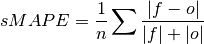
Parameters: - forecast (xarray object) – Forecast.
- verif (xarray object) – Verification data.
- dim (str) – Dimension(s) to perform metric over. Automatically set by compute function.
- weights (xarray object, optional) – Weights to apply over dimension. Defaults to
None. - skipna (bool, optional) – If True, skip NaNs over dimension being applied to.
Defaults to
False.
- Details:
minimum 0.0 maximum 1.0 perfect 0.0 orientation negative
See also
- xskillscore.smape
Unbiased Anomaly Correlation Coefficient (uACC)
# Enter any of the below keywords in ``metric=...`` for the compute functions.
In [18]: print(f"\n\nKeywords: {metric_aliases['uacc']}")


Keywords: ['uacc']
-
climpred.metrics._uacc(forecast, verif, dim=None, **metric_kwargs)[source]¶ Bushuk’s unbiased Anomaly Correlation Coefficient (uACC).
This is typically used in perfect model studies. Because the perfect model Anomaly Correlation Coefficient (ACC) is strongly state dependent, a standard ACC (e.g. one computed using
pearson_r) will be highly sensitive to the set of start dates chosen for the perfect model study. The Mean Square Skill Score (MSSS) can be related directly to the ACC asMSSS = ACC^(2)(see Murphy 1988 and Bushuk et al. 2019), so the unbiased ACC can be derived asuACC = sqrt(MSSS).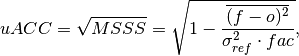
where
is 1 when using comparisons involving the ensemble mean (m2e,e2c,e2o) and 2 when using comparisons involving individual ensemble members (m2c,m2m,m2o). See_get_norm_factor().Note
Because of the square root involved, any negative
MSSSvalues are automatically converted to NaNs.Parameters: - forecast (xarray object) – Forecast.
- verif (xarray object) – Verification data.
- dim (str) – Dimension(s) to perform metric over. Automatically set by compute function.
- weights (xarray object, optional) – Weights to apply over dimension. Defaults to
None. - skipna (bool, optional) – If True, skip NaNs over dimension being applied to.
Defaults to
False. - comparison (str) – Name comparison needed for normalization factor
fac, see_get_norm_factor()(Handled internally by the compute functions)
- Details:
minimum 0.0 maximum 1.0 perfect 1.0 orientation positive better than climatology > 0.0 equal to climatology 0.0 - Reference:
- Bushuk, Mitchell, Rym Msadek, Michael Winton, Gabriel Vecchi, Xiaosong Yang, Anthony Rosati, and Rich Gudgel. “Regional Arctic Sea–Ice Prediction: Potential versus Operational Seasonal Forecast Skill.” Climate Dynamics, June 9, 2018. https://doi.org/10/gd7hfq.
- Allan H. Murphy. Skill Scores Based on the Mean Square Error and Their Relationships to the Correlation Coefficient. Monthly Weather Review, 116(12):2417–2424, December 1988. https://doi.org/10/fc7mxd.
Murphy Decomposition Metrics
Metrics derived in [Murphy1988] which decompose the MSESS into a correlation term,
a conditional bias term, and an unconditional bias term. See
https://www-miklip.dkrz.de/about/murcss/ for a walk through of the decomposition.
Standard Ratio
# Enter any of the below keywords in ``metric=...`` for the compute functions.
In [19]: print(f"\n\nKeywords: {metric_aliases['std_ratio']}")


Keywords: ['std_ratio']
-
climpred.metrics._std_ratio(forecast, verif, dim=None, **metric_kwargs)[source]¶ Ratio of standard deviations of the forecast over the verification data.
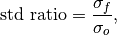
where
and are the standard deviations of the
forecast and the verification data over the experimental period, respectively.Parameters: - forecast (xarray object) – Forecast.
- verif (xarray object) – Verification data.
- dim (str) – Dimension(s) to perform metric over. Automatically set by compute functions.
- Details:
minimum 0.0 maximum ∞ perfect 1.0 orientation N/A - Reference:
Conditional Bias
# Enter any of the below keywords in ``metric=...`` for the compute functions.
In [20]: print(f"\n\nKeywords: {metric_aliases['conditional_bias']}")


Keywords: ['conditional_bias', 'c_b', 'cond_bias']
-
climpred.metrics._conditional_bias(forecast, verif, dim=None, **metric_kwargs)[source]¶ Conditional bias between forecast and verification data.
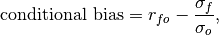
where
and are the standard deviations of the
forecast and verification data over the experimental period, respectively.Parameters: - forecast (xarray object) – Forecast.
- verif (xarray object) – Verification data.
- dim (str) – Dimension(s) to perform metric over. Automatically set by compute functions.
- Details:
minimum -∞ maximum 1.0 perfect 0.0 orientation negative - Reference:
Unconditional Bias
# Enter any of the below keywords in ``metric=...`` for the compute functions.
In [21]: print(f"\n\nKeywords: {metric_aliases['unconditional_bias']}")


Keywords: ['unconditional_bias', 'u_b', 'bias']
Simple bias of the forecast minus the observations.
-
climpred.metrics._unconditional_bias(forecast, verif, dim=None, **metric_kwargs)[source]¶ Unconditional bias.

Parameters: - forecast (xarray object) – Forecast.
- verif (xarray object) – Verification data.
- dim (str) – Dimension(s) to perform metric over. Automatically set by compute functions.
- Details:
minimum -∞ maximum ∞ perfect 0.0 orientation negative - Reference:
Bias Slope
# Enter any of the below keywords in ``metric=...`` for the compute functions.
In [22]: print(f"\n\nKeywords: {metric_aliases['bias_slope']}")


Keywords: ['bias_slope']
-
climpred.metrics._bias_slope(forecast, verif, dim=None, **metric_kwargs)[source]¶ Bias slope between verification data and forecast standard deviations.
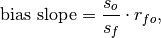
where
 is the Pearson product-moment correlation between the forecast
and the verification data and
is the Pearson product-moment correlation between the forecast
and the verification data and  and
and  are the standard
deviations of the verification data and forecast over the experimental period,
respectively.
are the standard
deviations of the verification data and forecast over the experimental period,
respectively.Parameters: - forecast (xarray object) – Forecast.
- verif (xarray object) – Verification data.
- dim (str) – Dimension(s) to perform metric over. Automatically set by compute functions.
- Details:
minimum 0.0 maximum ∞ perfect 1.0 orientation negative - Reference:
Murphy’s Mean Square Error Skill Score
# Enter any of the below keywords in ``metric=...`` for the compute functions.
In [23]: print(f"\n\nKeywords: {metric_aliases['msess_murphy']}")


Keywords: ['msess_murphy', 'msss_murphy']
-
climpred.metrics._msess_murphy(forecast, verif, dim=None, **metric_kwargs)[source]¶ Murphy’s Mean Square Error Skill Score (MSESS).
![MSESS_{Murphy} = r_{fo}^2 - [\text{conditional bias}]^2 - [\frac{\text{(unconditional) bias}}{\sigma_o}]^2,](_images/math/f4432517a8001eafced551d2c0377895ca11ab92.png)
where
 represents the Pearson product-moment correlation
coefficient between the forecast and verification data and
represents the standard deviation of the verification data over the experimental
period. See
represents the Pearson product-moment correlation
coefficient between the forecast and verification data and
represents the standard deviation of the verification data over the experimental
period. See conditional_biasandunconditional_biasfor their respective formulations.Parameters: - forecast (xarray object) – Forecast.
- verif (xarray object) – Verification data.
- dim (str) – Dimension(s) to perform metric over. Automatically set by compute function.
- weights (xarray object, optional) – Weights to apply over dimension. Defaults to
None. - skipna (bool, optional) – If True, skip NaNs over dimension being applied to.
Defaults to
False.
- Details:
minimum -∞ maximum 1.0 perfect 1.0 orientation positive
See also
- climpred.pearson_r
- climpred.conditional_bias
- climpred.unconditional_bias
- Reference:
- https://www-miklip.dkrz.de/about/murcss/
- Murphy, Allan H. “Skill Scores Based on the Mean Square Error and Their Relationships to the Correlation Coefficient.” Monthly Weather Review 116, no. 12 (December 1, 1988): 2417–24. https://doi.org/10/fc7mxd.
Probabilistic
Probabilistic metrics include the spread of the ensemble simulations in their calculations and assign a probability value between 0 and 1 to their forecasts [Jolliffe2011].
Continuous Ranked Probability Score (CRPS)
# Enter any of the below keywords in ``metric=...`` for the compute functions.
In [24]: print(f"\n\nKeywords: {metric_aliases['crps']}")


Keywords: ['crps']
-
climpred.metrics._crps(forecast, verif, **metric_kwargs)[source]¶ Continuous Ranked Probability Score (CRPS).
The CRPS can also be considered as the probabilistic Mean Absolute Error (
mae). It compares the empirical distribution of an ensemble forecast to a scalar observation. Smaller scores indicate better skill.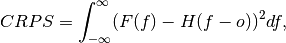
where
 is the cumulative distribution function (CDF) of the forecast
(since the verification data are not assigned a probability), and H() is the
Heaviside step function where the value is 1 if the argument is positive (i.e., the
forecast overestimates verification data) or zero (i.e., the forecast equals
verification data) and is 0 otherwise (i.e., the forecast is less than verification
data).
is the cumulative distribution function (CDF) of the forecast
(since the verification data are not assigned a probability), and H() is the
Heaviside step function where the value is 1 if the argument is positive (i.e., the
forecast overestimates verification data) or zero (i.e., the forecast equals
verification data) and is 0 otherwise (i.e., the forecast is less than verification
data).Note
The CRPS is expressed in the same unit as the observed variable. It generalizes the Mean Absolute Error (MAE), and reduces to the MAE if the forecast is determinstic.
Parameters: - forecast (xr.object) – Forecast with member dim.
- verif (xr.object) – Verification data without member dim.
- metric_kwargs (xr.object) – If provided, the CRPS is calculated exactly with the assigned probability weights to each forecast. Weights should be positive, but do not need to be normalized. By default, each forecast is weighted equally.
- Details:
minimum 0.0 maximum ∞ perfect 0.0 orientation negative - Reference:
- Matheson, James E., and Robert L. Winkler. “Scoring Rules for Continuous Probability Distributions.” Management Science 22, no. 10 (June 1, 1976): 1087–96. https://doi.org/10/cwwt4g.
- https://www.lokad.com/continuous-ranked-probability-score
See also
- properscoring.crps_ensemble
- xskillscore.crps_ensemble
Continuous Ranked Probability Skill Score (CRPSS)
# Enter any of the below keywords in ``metric=...`` for the compute functions.
In [25]: print(f"\n\nKeywords: {metric_aliases['crpss']}")


Keywords: ['crpss']
-
climpred.metrics._crpss(forecast, verif, **metric_kwargs)[source]¶ Continuous Ranked Probability Skill Score.
This can be used to assess whether the ensemble spread is a useful measure for the forecast uncertainty by comparing the CRPS of the ensemble forecast to that of a reference forecast with the desired spread.
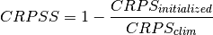
Note
When assuming a Gaussian distribution of forecasts, use default
gaussian=True. If not gaussian, you may specify the distribution type, xmin/xmax/tolerance for integration (see xskillscore.crps_quadrature).Parameters: - forecast (xr.object) – Forecast with
memberdim. - verif (xr.object) – Verification data without
memberdim. - gaussian (bool, optional) – If
True, assum Gaussian distribution for baseline skill. Defaults toTrue. - cdf_or_dist (scipy.stats) – Function which returns the cumulative density of the
forecast at value x. This can also be an object with
a callable
cdf()method such as ascipy.stats.distributionobject. Defaults toscipy.stats.norm. - xmin (float) – Lower bounds for integration. Only use if not assuming Gaussian.
- xmax (float) –
- tol (float, optional) – The desired accuracy of the CRPS. Larger values will
speed up integration. If
tolis set toNone, bounds errors or integration tolerance errors will be ignored. Only use if not assuming Gaussian.
- Details:
minimum -∞ maximum 1.0 perfect 1.0 orientation positive better than climatology > 0.0 worse than climatology < 0.0 - Reference:
- Matheson, James E., and Robert L. Winkler. “Scoring Rules for Continuous Probability Distributions.” Management Science 22, no. 10 (June 1, 1976): 1087–96. https://doi.org/10/cwwt4g.
- Gneiting, Tilmann, and Adrian E Raftery. “Strictly Proper Scoring Rules, Prediction, and Estimation.” Journal of the American Statistical Association 102, no. 477 (March 1, 2007): 359–78. https://doi.org/10/c6758w.
Example
>>> compute_perfect_model(ds, control, metric='crpss')
>>> compute_perfect_model(ds, control, metric='crpss', gaussian=False,
                          cdf_or_dist=scipy.stats.norm, xminimum=-10,
                          xmaximum=10, tol=1e-6)
See also
- properscoring.crps_ensemble
- xskillscore.crps_ensemble
- forecast (xr.object) – Forecast with
Continuous Ranked Probability Skill Score Ensemble Spread
# Enter any of the below keywords in ``metric=...`` for the compute functions.
In [26]: print(f"\n\nKeywords: {metric_aliases['crpss_es']}")


Keywords: ['crpss_es']
-
climpred.metrics._crpss_es(forecast, verif, **metric_kwargs)[source]¶ Continuous Ranked Probability Skill Score Ensemble Spread.
If the ensemble variance is smaller than the observed
mse, the ensemble is said to be under-dispersive (or overconfident). An ensemble with variance larger than the verification data indicates one that is over-dispersive (underconfident).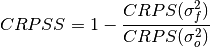
Parameters: - forecast (xr.object) – Forecast with
memberdim. - verif (xr.object) – Verification data without
memberdim. - weights (xarray object, optional) – Weights to apply over dimension. Defaults to
None. - skipna (bool, optional) – If True, skip NaNs over dimension being applied to.
Defaults to
False.
- Details:
minimum -∞ maximum 0.0 perfect 0.0 orientation positive under-dispersive > 0.0 over-dispersive < 0.0 - Reference:
- Kadow, Christopher, Sebastian Illing, Oliver Kunst, Henning W. Rust, Holger Pohlmann, Wolfgang A. Müller, and Ulrich Cubasch. “Evaluation of Forecasts by Accuracy and Spread in the MiKlip Decadal Climate Prediction System.” Meteorologische Zeitschrift, December 21, 2016, 631–43. https://doi.org/10/f9jrhw.
- Range:
- perfect: 0
- else: negative
- forecast (xr.object) – Forecast with
Brier Score
# Enter any of the below keywords in ``metric=...`` for the compute functions.
In [27]: print(f"\n\nKeywords: {metric_aliases['brier_score']}")


Keywords: ['brier_score', 'brier', 'bs']
-
climpred.metrics._brier_score(forecast, verif, **metric_kwargs)[source]¶ Brier Score.
The Mean Square Error (
mse) of probabilistic two-category forecasts where the verification data are either 0 (no occurrence) or 1 (occurrence) and forecast probability may be arbitrarily distributed between occurrence and non-occurrence. The Brier Score equals zero for perfect (single-valued) forecasts and one for forecasts that are always incorrect.
where
 is the forecast probability of
  .
.Note
The Brier Score requires that the observation is binary, i.e., can be described as one (a “hit”) or zero (a “miss”).
Parameters: - forecast (xr.object) – Forecast with
memberdim. - verif (xr.object) – Verification data without
memberdim. - func (function) – Function to be applied to verification data and forecasts
and then
mean('member')to get forecasts and verification data in interval [0,1].
- Details:
minimum 0.0 maximum 1.0 perfect 0.0 orientation negative - Reference:
- Brier, Glenn W. Verification of forecasts expressed in terms of probability.” Monthly Weather Review 78, no. 1 (1950). https://doi.org/10.1175/1520-0493(1950)078<0001:VOFEIT>2.0.CO;2.
- https://www.nws.noaa.gov/oh/rfcdev/docs/ Glossary_Forecast_Verification_Metrics.pdf
See also
- properscoring.brier_score
- xskillscore.brier_score
Example
>>> def pos(x): return x > 0
>>> compute_perfect_model(ds, control, metric='brier_score', func=pos)
- forecast (xr.object) – Forecast with
Threshold Brier Score
# Enter any of the below keywords in ``metric=...`` for the compute functions.
In [28]: print(f"\n\nKeywords: {metric_aliases['threshold_brier_score']}")


Keywords: ['threshold_brier_score', 'tbs']
-
climpred.metrics._threshold_brier_score(forecast, verif, **metric_kwargs)[source]¶ Brier score of an ensemble for exceeding given thresholds.
where
 is the cumulative distribution
function (CDF) of the forecast distribution
is the cumulative distribution
function (CDF) of the forecast distribution  ,
,  is a point estimate
of the true observation (observational error is neglected),
is a point estimate
of the true observation (observational error is neglected),  denotes the
Brier score and
denotes the
Brier score and  denotes the Heaviside step function, which we define
here as equal to 1 for
denotes the Heaviside step function, which we define
here as equal to 1 for  and 0 otherwise.
Parameters: - forecast (xr.object) – Forecast with
memberdim. - verif (xr.object) – Verification data without
memberdim. - threshold (int, float, xr.object) – Threshold to check exceedance, see properscoring.threshold_brier_score.
- Details:
minimum 0.0 maximum 1.0 perfect 0.0 orientation negative - Reference:
- Brier, Glenn W. Verification of forecasts expressed in terms of probability.” Monthly Weather Review 78, no. 1 (1950). https://doi.org/10.1175/1520-0493(1950)078<0001:VOFEIT>2.0.CO;2.
See also
- properscoring.threshold_brier_score
- xskillscore.threshold_brier_score
Example
>>> compute_perfect_model(ds, control,
                          metric='threshold_brier_score', threshold=.5)
- forecast (xr.object) – Forecast with
User-defined metrics
You can also construct your own metrics via the climpred.metrics.Metric
class.
Metric(name, function, positive, …[, …]) |
Master class for all metrics. |
First, write your own metric function, similar to the existing ones with required
arguments forecast, observations, dim=None, and **metric_kwargs:
from climpred.metrics import Metric

def _my_msle(forecast, observations, dim=None, **metric_kwargs):
    """Mean squared logarithmic error (MSLE).
    https://peltarion.com/knowledge-center/documentation/modeling-view/build-an-ai-model/loss-functions/mean-squared-logarithmic-error."""
    return ( (np.log(forecast + 1) + np.log(observations + 1) ) ** 2).mean(dim)
Then initialize this metric function with climpred.metrics.Metric:
_my_msle = Metric(
    name='my_msle',
    function=_my_msle,
    probabilistic=False,
    positive=False,
    unit_power=0,
    )
Finally, compute skill based on your own metric:
skill = compute_perfect_model(ds, control, metric=_my_msle)
Once you come up with an useful metric for your problem, consider contributing this metric to climpred, so all users can benefit from your metric, see contributing.
References
| [Jolliffe2011] | (1, 2) Ian T. Jolliffe and David B. Stephenson. Forecast Verification: A Practitioner’s Guide in Atmospheric Science. John Wiley & Sons, Ltd, Chichester, UK, December 2011. ISBN 978-1-119-96000-3 978-0-470-66071-3. URL: http://doi.wiley.com/10.1002/9781119960003. |
| [Murphy1988] | Allan H. Murphy. Skill Scores Based on the Mean Square Error and Their Relationships to the Correlation Coefficient. Monthly Weather Review, 116(12):2417–2424, December 1988. https://doi.org/10/fc7mxd. |