Significance Testing
This demo shows how to handle significance testing from a functional perspective of climpred. In the future, we will have a robust significance testing framework inplemented with HindcastEnsemble and PerfectModelEnsemble objects.
[ ]:
import xarray as xr
from climpred.tutorial import load_dataset
from climpred.stats import rm_poly
from climpred.prediction import compute_hindcast, compute_perfect_model
from climpred.bootstrap import bootstrap_hindcast, bootstrap_perfect_model
import matplotlib.pyplot as plt

import warnings

warnings.filterwarnings("ignore")
[2]:
# load data
v = "SST"
hind = load_dataset("CESM-DP-SST")[v]
hind.lead.attrs["units"] = "years"

hist = load_dataset("CESM-LE")[v]
hist = hist - hist.mean()

obs = load_dataset("ERSST")[v]
obs = obs - obs.mean()
[3]:
# align times
hind["init"] = xr.cftime_range(
    start=str(hind.init.min().astype("int").values), periods=hind.init.size, freq="YS"
)
hist["time"] = xr.cftime_range(
    start=str(hist.time.min().astype("int").values), periods=hist.time.size, freq="YS"
)
obs["time"] = xr.cftime_range(
    start=str(obs.time.min().astype("int").values), periods=obs.time.size, freq="YS"
)
[4]:
# view the data
hind.sel(lead=1).mean("member").plot(label="CESM-DPLE hindcast lead=1")
hist.mean("member").plot(label="CESM-LE historical")
obs.plot(label="ERSST observations")
plt.legend()
plt.title(f"global mean {v}")
plt.show()
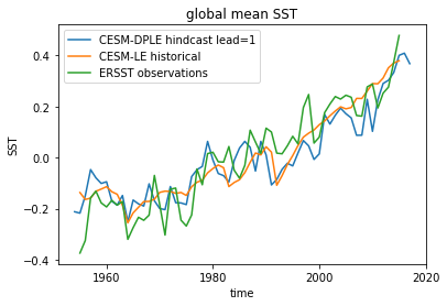
Here we see the strong trend due to climate change. This trend is not linear but rather quadratic. Because we often aim to prediction natural variations and not specifically the external forcing in initialized predictions, we remove the 2nd-order trend from each dataset along a time axis.
[5]:
order = 2
hind = rm_poly(hind, dim="init", order=order)
hist = rm_poly(hist, dim="time", order=order)
obs = rm_poly(obs, dim="time", order=order)
# lead attrs is lost in rm_poly
hind.lead.attrs["units"] = "years"
[6]:
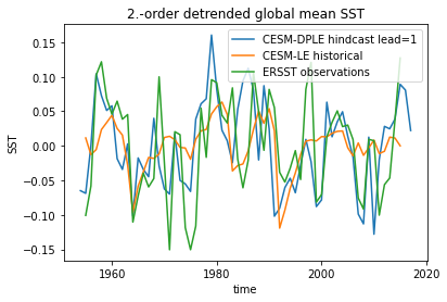
hind.sel(lead=1).mean("member").plot(label="CESM-DPLE hindcast lead=1")
hist.mean("member").plot(label="CESM-LE historical")
obs.plot(label="ERSST observations")
plt.legend()
plt.title(f"{order}.-order detrended global mean {v}")
plt.show()
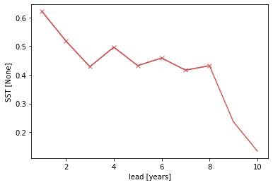
p value for temporal correlations
For correlation metrics the associated p-value checks whether the correlation is significantly different from zero incorporating reduced degrees of freedom due to temporal autocorrelation.
[7]:
# level that initialized ensembles are significantly better than other forecast skills
sig = 0.05
[8]:
acc = compute_hindcast(hind, obs, metric="pearson_r", comparison="e2r")

acc_p_value = compute_hindcast(hind, obs, metric="pearson_r_eff_p_value", comparison="e2r")
[9]:
init_color = "indianred"
acc.plot(c=init_color)
acc.where(acc_p_value <= sig).plot(marker="x", c=init_color)
[9]:
[<matplotlib.lines.Line2D at 0x1288a69b0>]
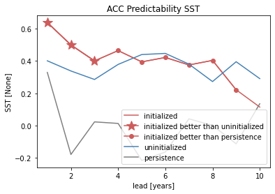
Bootstrapping with replacement
Bootstrapping significance relies on resampling the underlying data with replacement for a large number of iterations as proposed by the decadal prediction framework of Goddard et al. 2013. We just use 20 iterations here to demonstrate the functionality.
[10]:
%%time
bootstrapped_acc = bootstrap_hindcast(
    hind, hist, obs, metric="pearson_r", comparison="e2r", iterations=500, sig=95
)
CPU times: user 1.7 s, sys: 46.4 ms, total: 1.75 s
Wall time: 1.77 s
[11]:
bootstrapped_acc.coords
[11]:
Coordinates:
  * kind     (kind) object 'init' 'pers' 'uninit'
  * lead     (lead) int64 1 2 3 4 5 6 7 8 9 10
  * results  (results) <U7 'skill' 'p' 'low_ci' 'high_ci'
bootstrap_acc contains for the three different kinds of predictions: - init for the initialized hindcast hind and describes skill due to initialization and external forcing - uninit for the uninitialized historical hist and approximates skill from external forcing - pers for the reference forecast computed by baseline_compute, which defaults to compute_persistence
for different results: - skill: skill values - p: p value - low_ci and high_ci: high and low ends of confidence intervals based on significance threshold sig
[12]:
init_skill = bootstrapped_acc.sel(results="skill", kind="init")
init_better_than_uninit = init_skill.where(
    bootstrapped_acc.sel(results="p", kind="uninit") <= sig
)
init_better_than_persistence = init_skill.where(
    bootstrapped_acc.sel(results="p", kind="pers") <= sig
)
[13]:
# create a plot by hand
bootstrapped_acc.sel(results="skill", kind="init").plot(
    c=init_color, label="initialized"
)
init_better_than_uninit.plot(
    c=init_color,
    marker="*",
    markersize=15,
    label="initialized better than uninitialized",
)
init_better_than_persistence.plot(
    c=init_color, marker="o", label="initialized better than persistence"
)
bootstrapped_acc.sel(results="skill", kind="uninit").plot(
    c="steelblue", label="uninitialized"
)
bootstrapped_acc.sel(results="skill", kind="pers").plot(c="gray", label="persistence")
plt.title(f"ACC Predictability {v}")
plt.legend(loc="lower right")
[13]:
<matplotlib.legend.Legend at 0x12a1f4320>
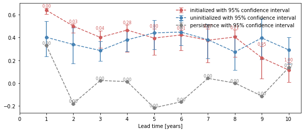
[14]:
# use climpred convenience plotting function
from climpred.graphics import plot_bootstrapped_skill_over_leadyear

plot_bootstrapped_skill_over_leadyear(bootstrapped_acc)
[14]:
<matplotlib.axes._subplots.AxesSubplot at 0x1264bdc88>
Field significance
Using esmtools.testing.multipletests to control the false discovery rate (FDR) from the above obtained p-values in geospatial data.
[15]:
v = "tos"
ds3d = load_dataset("MPI-PM-DP-3D")[v]
ds3d.lead.attrs["unit"] = "years"
control3d = load_dataset("MPI-control-3D")[v]
p value for temporal correlations
[16]:
# ACC skill
acc3d = compute_perfect_model(ds3d, control3d, metric="pearson_r", comparison="m2e")

# ACC_p_value skill
acc_p_3d = compute_perfect_model(
    ds3d, control3d, metric="pearson_r_p_value", comparison="m2e"
)
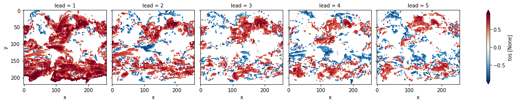
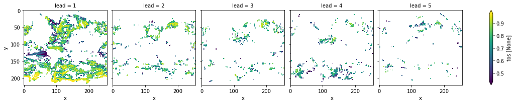
[17]:
# mask init skill where not significant
acc3d.where(acc_p_3d <= sig).plot(col="lead", robust=True, yincrease=False)
[17]:
<xarray.plot.facetgrid.FacetGrid at 0x128845b00>
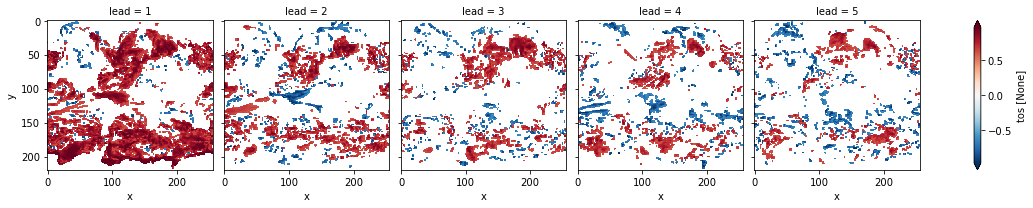
[18]:
# apply FDR Benjamini-Hochberg
# relies on esmtools https://github.com/bradyrx/esmtools
from esmtools.testing import multipletests

_, acc_p_3d_fdr_corr = multipletests(acc_p_3d, method="fdr_bh", alpha=sig)
[19]:
# mask init skill where not significant on corrected p-values
acc3d.where(acc_p_3d_fdr_corr <= sig).plot(col="lead", robust=True, yincrease=False)
[19]:
<xarray.plot.facetgrid.FacetGrid at 0x122e5d2e8>
[20]:
# difference due to FDR Benjamini-Hochberg
(acc_p_3d_fdr_corr - acc_p_3d).plot(col="lead", robust=True, yincrease=False)
[20]:
<xarray.plot.facetgrid.FacetGrid at 0x123048dd8>
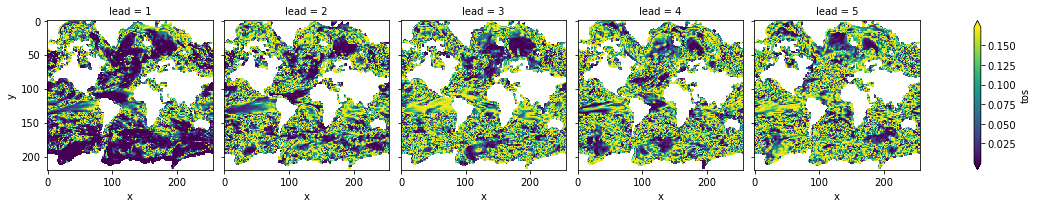
FDR Benjamini-Hochberg increases the p-value and therefore reduces the number of significant grid cells.
Bootstrapping with replacement
[37]:
%%time
bootstrapped_acc_3d = bootstrap_perfect_model(
    ds3d, control3d, metric="pearson_r", comparison="m2e", iterations=10
)
CPU times: user 22.2 s, sys: 12.7 s, total: 35 s
Wall time: 42.5 s
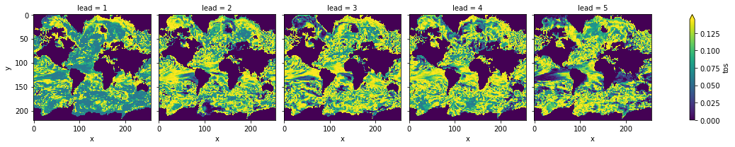
[46]:
# mask init skill where not significant
bootstrapped_acc_3d.sel(kind="init", results="skill").where(
    bootstrapped_acc_3d.sel(kind="uninit", results="p") <= sig
).plot(col="lead", robust=True, yincrease=False)
[46]:
<xarray.plot.facetgrid.FacetGrid at 0x141955400>
[66]:
# apply FDR Benjamini-Hochberg
_, bootstrapped_acc_p_3d_fdr_corr = multipletests(
    bootstrapped_acc_3d.sel(kind="uninit", results="p"), method="fdr_bh", alpha=sig
)
[75]:
# mask init skill where not significant on corrected p-values
bootstrapped_acc_3d.sel(kind="init", results="skill").where(
    bootstrapped_acc_p_3d_fdr_corr <= sig*2
).plot(col="lead", robust=True, yincrease=False)
[75]:
<xarray.plot.facetgrid.FacetGrid at 0x157e438d0>

[76]:
# difference due to FDR Benjamini-Hochberg
(
    bootstrapped_acc_p_3d_fdr_corr - bootstrapped_acc_3d.sel(kind="uninit", results="p")
).plot(col="lead", robust=True, yincrease=False)
[76]:
<xarray.plot.facetgrid.FacetGrid at 0x158b34048>
FDR Benjamini-Hochberg increases the p-value and therefore reduces the number of significant grid cells.