Significance Testing
This demo shows how to handle significance testing from a functional perspective of climpred. In the future, we will have a robust significance testing framework inplemented with HindcastEnsemble and PerfectModelEnsemble objects.
[1]:
# linting
%load_ext nb_black
%load_ext lab_black
[2]:
import xarray as xr
import numpy as np
from climpred.tutorial import load_dataset
from climpred import HindcastEnsemble, PerfectModelEnsemble
import matplotlib.pyplot as plt
[3]:
# load data
v = "SST"
hind = load_dataset("CESM-DP-SST")[v]
hind.lead.attrs["units"] = "years"

hist = load_dataset("CESM-LE")[v]
hist = hist - hist.mean()

obs = load_dataset("ERSST")[v]
obs = obs - obs.mean()
[4]:
hindcast = HindcastEnsemble(hind)
hindcast = hindcast.add_uninitialized(hist)
hindcast = hindcast.add_observations(obs)

hindcast.plot()
/Users/aaron.spring/Coding/climpred/climpred/utils.py:122: UserWarning: Assuming annual resolution due to numeric inits. Change init to a datetime if it is another resolution.
  warnings.warn(
[4]:
<AxesSubplot:xlabel='time', ylabel='SST'>
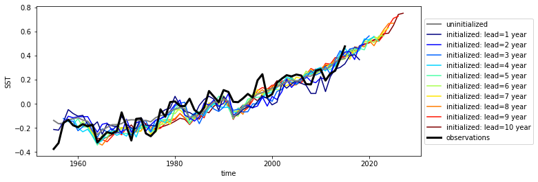
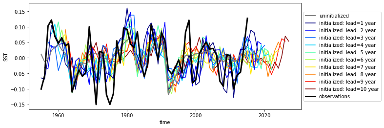
Here we see the strong trend due to climate change. This trend is not linear but rather quadratic. Because we often aim to prediction natural variations and not specifically the external forcing in initialized predictions, we remove the 2nd-order trend from each dataset along a time axis.
[5]:
from climpred.stats import rm_poly

hindcast = hindcast.map(rm_poly, dim="init_or_time", deg=2)

hindcast.plot()
[5]:
<AxesSubplot:xlabel='time', ylabel='SST'>
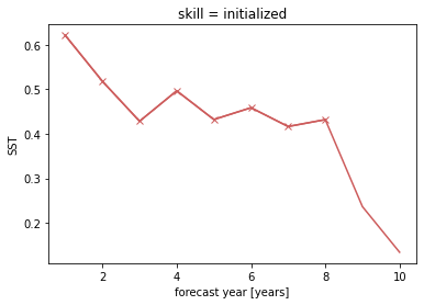
p value for temporal correlations
For correlation metrics the associated p-value checks whether the correlation is significantly different from zero incorporating reduced degrees of freedom due to temporal autocorrelation.
[6]:
# level that initialized ensembles are significantly better than other forecast skills
sig = 0.05
[7]:
acc = hindcast.verify(
    metric="pearson_r", comparison="e2o", dim="init", alignment="same_verif"
)["SST"]
acc_p_value = hindcast.verify(
    metric="pearson_r_eff_p_value", comparison="e2o", dim="init", alignment="same_verif"
)["SST"]
[8]:
init_color = "indianred"
acc.plot(c=init_color)
acc.where(acc_p_value <= sig).plot(marker="x", c=init_color)
[8]:
[<matplotlib.lines.Line2D at 0x7fc45afd1280>]
Bootstrapping with replacement
Bootstrapping significance relies on resampling the underlying data with replacement for a large number of iterations as proposed by the decadal prediction framework of Goddard et al. 2013. We just use 20 iterations here to demonstrate the functionality.
[9]:
%%time

bootstrapped_acc = hindcast.bootstrap(
    metric="pearson_r",
    comparison="e2r",
    dim="init",
    alignment="same_verif",
    iterations=500,
    sig=95,
    reference=["uninitialized", "persistence", "climatology"],
)
CPU times: user 1.17 s, sys: 173 ms, total: 1.34 s
Wall time: 1.4 s
[10]:
bootstrapped_acc.coords
[10]:
Coordinates:
  * lead     (lead) int32 1 2 3 4 5 6 7 8 9 10
  * results  (results) <U12 'verify skill' 'p' 'low_ci' 'high_ci'
  * skill    (skill) <U13 'initialized' 'uninitialized' ... 'climatology'
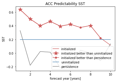
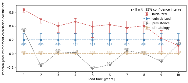
bootstrap_acc contains skill of initialized and reference given by reference: - initialized for the initialized hindcast hind and describes skill due to initialization and external forcing - uninitialized for the uninitialized historical hist and approximates skill from external forcing - persistence for the reference persistence forecast
for different results: - verify skill: skill values - p: p value that reference forecast is better than initialized - low_ci and high_ci: high and low ends of confidence intervals based on significance threshold sig
[11]:
init_skill = bootstrapped_acc[v].sel(results="verify skill", skill="initialized")
init_better_than_uninit = init_skill.where(
    bootstrapped_acc[v].sel(results="p", skill="uninitialized") <= sig
)
init_better_than_persistence = init_skill.where(
    bootstrapped_acc[v].sel(results="p", skill="persistence") <= sig
)
[12]:
# create a plot by hand
bootstrapped_acc[v].sel(results="verify skill", skill="initialized").plot(
    c=init_color, label="initialized"
)
init_better_than_uninit.plot(
    c=init_color,
    marker="*",
    markersize=15,
    label="initialized better than uninitialized",
)
init_better_than_persistence.plot(
    c=init_color, marker="o", label="initialized better than persistence"
)
bootstrapped_acc[v].sel(results="verify skill", skill="uninitialized").plot(
    c="steelblue", label="uninitialized"
)
bootstrapped_acc[v].sel(results="verify skill", skill="persistence").plot(
    c="gray", label="persistence"
)
plt.title(f"ACC Predictability {v}")
plt.legend(loc="lower right")
[12]:
<matplotlib.legend.Legend at 0x7fc45aff7880>
[13]:
# use climpred convenience plotting function
from climpred.graphics import plot_bootstrapped_skill_over_leadyear

plot_bootstrapped_skill_over_leadyear(bootstrapped_acc)
[13]:
<AxesSubplot:xlabel='Lead time [years]', ylabel='Pearson product-moment correlation coefficient'>
Field significance
Using esmtools.testing.multipletests to control the false discovery rate (FDR) from the above obtained p-values in geospatial data.
[14]:
v = "tos"
ds3d = load_dataset("MPI-PM-DP-3D")[v]
ds3d.lead.attrs["unit"] = "years"
control3d = load_dataset("MPI-control-3D")[v]
[15]:
pm = PerfectModelEnsemble(ds3d)
pm = pm.add_control(control3d)
/Users/aaron.spring/Coding/climpred/climpred/utils.py:122: UserWarning: Assuming annual resolution due to numeric inits. Change init to a datetime if it is another resolution.
  warnings.warn(
p value for temporal correlations
Lets first calculate the Pearson’s Correlation p-value and then correct afterwards by FDR.
[16]:
acc3d = pm.verify(metric="pearson_r", comparison="m2e", dim=["init", "member"])[v]
acc_p_3d = pm.verify(
    metric="pearson_r_p_value", comparison="m2e", dim=["init", "member"]
)[v]
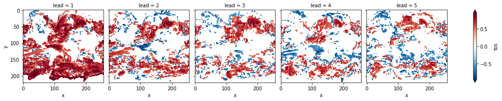
[17]:
# mask init skill where not significant
acc3d.where(acc_p_3d <= sig).plot(col="lead", robust=True, yincrease=False, x="x")
[17]:
<xarray.plot.facetgrid.FacetGrid at 0x7fc46034f1f0>
[18]:
# apply FDR Benjamini-Hochberg
# relies on esmtools https://github.com/bradyrx/esmtools
from esmtools.testing import multipletests

_, acc_p_3d_fdr_corr = multipletests(acc_p_3d, method="fdr_bh", alpha=sig)
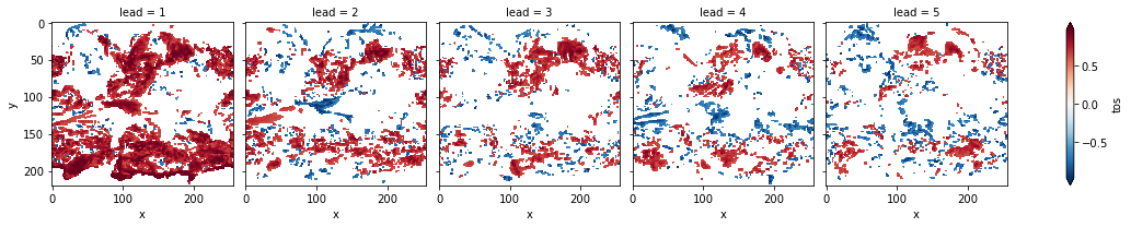
[19]:
# mask init skill where not significant on corrected p-values
acc3d.where(acc_p_3d_fdr_corr <= sig).plot(
    col="lead", robust=True, yincrease=False, x="x"
)
[19]:
<xarray.plot.facetgrid.FacetGrid at 0x7fc45af888e0>
[20]:
# difference due to FDR Benjamini-Hochberg
(acc_p_3d_fdr_corr - acc_p_3d).plot(col="lead", robust=True, yincrease=False, x="x")
[20]:
<xarray.plot.facetgrid.FacetGrid at 0x7fc445f69c40>
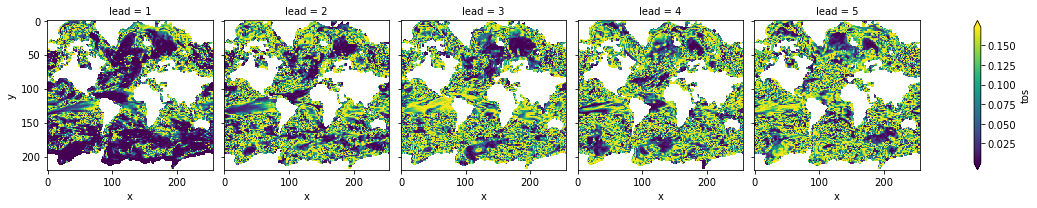
FDR Benjamini-Hochberg increases the p-value and therefore reduces the number of significant grid cells.
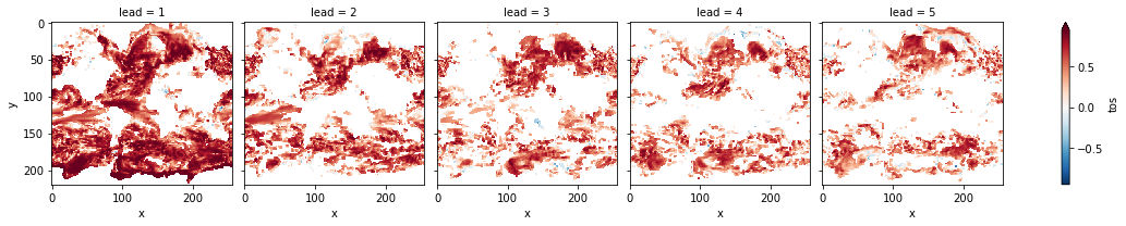
Bootstrapping with replacement
The same applies to bootstrapping with replacement. First calculate the pvalue that uninitialized are better than initialized forecasts. Then correct the FDR.
[21]:
%%time
bootstrapped_acc_3d = pm.bootstrap(metric="pearson_r", comparison="m2e", dim=['init', 'member'],
                                   iterations=10, reference='uninitialized')['tos']
/Users/aaron.spring/Coding/climpred/climpred/checks.py:229: UserWarning: Consider chunking input `ds` along other dimensions than needed by algorithm, e.g. spatial dimensions, for parallelized performance increase.
  warnings.warn(
CPU times: user 9.99 s, sys: 3.02 s, total: 13 s
Wall time: 13.7 s
[22]:
# mask init skill where not significant
bootstrapped_acc_3d.sel(skill="initialized", results="verify skill").where(
    bootstrapped_acc_3d.sel(skill="uninitialized", results="p") <= sig
).plot(col="lead", robust=True, yincrease=False, x="x")
[22]:
<xarray.plot.facetgrid.FacetGrid at 0x7fc44684d970>

[23]:
# apply FDR Benjamini-Hochberg
_, bootstrapped_acc_p_3d_fdr_corr = multipletests(
    bootstrapped_acc_3d.sel(skill="uninitialized", results="p"),
    method="fdr_bh",
    alpha=sig,
)
[24]:
# mask init skill where not significant on corrected p-values
bootstrapped_acc_3d.sel(skill="initialized", results="verify skill").where(
    bootstrapped_acc_p_3d_fdr_corr <= sig * 2
).plot(col="lead", robust=True, yincrease=False, x="x")
[24]:
<xarray.plot.facetgrid.FacetGrid at 0x7fc44874ce80>
[25]:
# difference due to FDR Benjamini-Hochberg
(
    bootstrapped_acc_p_3d_fdr_corr
    - bootstrapped_acc_3d.sel(skill="uninitialized", results="p").where(
        bootstrapped_acc_3d.sel(skill="uninitialized", results="p")
    )
).plot(
    col="lead",
    robust=True,
    yincrease=False,
    x="x",
    cmap="RdBu_r",
    vmin=-0.04,
    vmax=0.04,
)
[25]:
<xarray.plot.facetgrid.FacetGrid at 0x7fc46030d070>
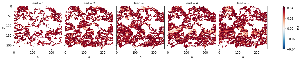
FDR Benjamini-Hochberg increases the p-value and therefore reduces the number of significant grid cells.
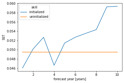
Coin test
Use xskillscore.sign_test to decide which forecast is better. Here we compare the initialized with the uninitialized forecast.
DelSole, T., & Tippett, M. K. (2016). Forecast Comparison Based on Random Walks. Monthly Weather Review, 144(2), 615–626. doi: 10/f782pf
[26]:
skill = hindcast.verify(
    metric="mae",
    comparison="e2o",
    dim=[],
    alignment="same_verif",
    reference="uninitialized",
).SST

# initialized skill is clearly better than historical skill
skill.mean("init").plot(hue="skill")
[26]:
[<matplotlib.lines.Line2D at 0x7fc2f8fdc370>,
 <matplotlib.lines.Line2D at 0x7fc2f8fdc460>]
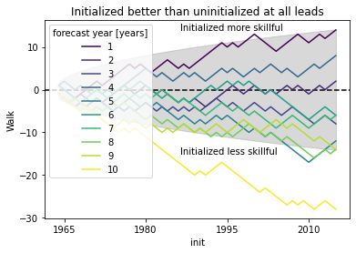
[27]:
from xskillscore import sign_test

# orientation is negative since lower scores are better for MAE
init_better_uninit, walk, confidence = sign_test(
    skill.sel(skill="initialized"),
    skill.sel(skill="uninitialized"),
    time_dim="init",
    orientation="negative",
    alpha=sig,
)
[28]:
plt.rcParams["legend.loc"] = "upper left"
plt.rcParams["axes.prop_cycle"] = plt.cycler(
    "color", plt.cm.viridis(np.linspace(0, 1, walk.lead.size))
)
# positive walk means forecast1 (here initialized) is better than forecast2 (uninitialized)
# skillful when colored line above gray line following a random walk
# this gives you the possibility to see which inits have better skill (positive step) than reference
# the final inital init shows the combined result over all inits as the sign_test is a `cumsum`
conf = confidence.isel(lead=0)  # confidence is identical here for all leads
plt.fill_between(conf.init.values, conf, -conf, color="gray", alpha=0.3)
plt.axhline(y=0, c="k", ls="--")
walk.plot(hue="lead")
plt.title("Initialized better than uninitialized at all leads")
plt.ylabel("Walk")
plt.annotate("Initialized more skillful", (-5000, 14), xycoords="data")
plt.annotate("Initialized less skillful", (-5000, -15), xycoords="data")
plt.show()
[ ]: