Demo of Perfect Model Predictability Functions

This demo demonstrates climpred’s capabilities for a perfect-model framework ensemble simulation.

What’s a perfect-model framework simulation?

A perfect-model framework uses a set of ensemble simulations that are based on a General Circulation Model (GCM) or Earth System Model (ESM) alone. There is no use of any reanalysis, reconstruction, or data product to initialize the decadal prediction ensemble. An arbitrary number of members are initialized from perturbed initial conditions (the “ensemble”), and the control simulation can be viewed as just another member.

How to compare predictability skill score: As no observational data interferes with the random climate evolution of the model, we cannot use an observation-based reference for computing skill scores. Therefore, we can compare the members with one another (m2m), against the ensemble mean (m2e), or against the control (m2c). We can also compare the ensemble mean to the control (e2c). See the comparisons page for more information.

When to use perfect-model frameworks:

• You don’t have a sufficiently long observational record to use as a reference.
• You want to avoid biases between model climatology and reanalysis climatology.
• You want to avoid sensitive reactions of biogeochemical cycles to disruptive changes in ocean physics due to assimilation.
• You want to delve into process understanding of predictability in a model without outside artifacts.

import warnings

import cartopy.crs as ccrs
import cartopy.feature as cfeature
%matplotlib inline
import matplotlib.pyplot as plt
import numpy as np
import xarray as xr

import climpred

warnings.filterwarnings("ignore")

Load sample data

Here we use a subset of ensembles and members from the MPI-ESM-LR (CMIP6 version) esmControl simulation of an early state. This corresponds to vga0214 from year 3000 to 3300.

1-dimensional output

Our 1D sample output contains datasets of time series of certain spatially averaged area (‘global’, ‘North_Atlantic’) and temporally averaged period (‘ym’, ‘DJF’, …) for some lead years (1, …, 20).

ds: The ensemble dataset of all members (1, …, 10), inits (initialization years: 3014, 3023, …, 3257), areas, periods, and lead years.

control: The control dataset with the same areas and periods, as well as the years 3000 to 3299.

ds = climpred.tutorial.load_dataset('MPI-PM-DP-1D')
control = climpred.tutorial.load_dataset('MPI-control-1D')

We’ll sub-select annual means (‘ym’) of sea surface temperature (‘tos’) in the North Atlantic.

varname = 'tos'
area = 'North_Atlantic'
period = 'ym'

ds = ds.sel(area=area, period=period)[varname]
control = control.sel(area=area, period=period)[varname]
ds = ds.reset_coords(drop=True)
control = control.reset_coords(drop=True)

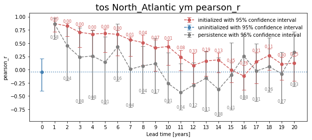
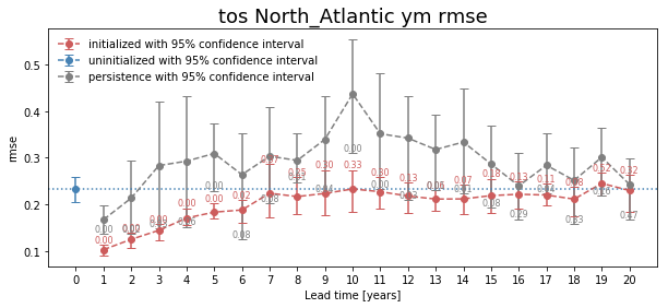
Bootstrapping with Replacement

Here, we bootstrap the ensemble with replacement [Goddard et al. 2013] to compare the initialized ensemble to an “uninitialized” counterpart and a persistence forecast. The visualization is based on those used in [Li et al. 2016]. The p-value demonstrates the probability that the uninitialized or persistence beats the initialized forecast based on N=100 bootstrapping with replacement.

for metric in ['pearson_r', 'rmse']:
    bootstrapped = climpred.bootstrap.bootstrap_perfect_model(ds,
                                                              control,
                                                              metric=metric,
                                                              comparison='m2e',
                                                              bootstrap=100,
                                                              sig=95)

    climpred.graphics.plot_bootstrapped_skill_over_leadyear(bootstrapped, sig)
    plt.title(' '.join([varname, area, period, metric]),fontsize=18)
    plt.ylabel(metric)
    plt.show()

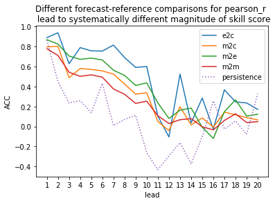
Computing Skill with Different Comparison Methods

Here, we use compute_perfect_model to compute the Anomaly Correlation Coefficient (ACC) with different comparison methods. This generates different ACC values by design. See the comparisons page for a description of the various ways to compute skill scores for a perfect-model framework.

for c in ['e2c','m2c','m2e','m2m']:
    climpred.prediction.compute_perfect_model(ds,
                                              control,
                                              metric='pearson_r',
                                              comparison=c).plot(label=c)
# Persistence computation for a baseline.
climpred.prediction.compute_persistence(ds, control).plot(label='persistence', ls=':')
plt.ylabel('ACC')
plt.xticks(np.arange(1,21))
plt.legend()
plt.title('Different forecast-reference comparisons for pearson_r \n lead to systematically different magnitude of skill score')
plt.show()

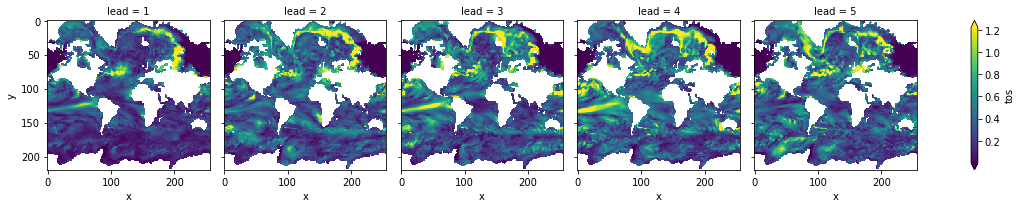
3-dimensional output (maps)

We also have some sample output that contains gridded time series on the curvilinear MPI grid. Our compute functions (compute_perfect_model, compute_persistence) are indifferent to any dimensions that exist in addition to init, member, and lead. In other words, the functions are set up to make these computations on a grid, if one includes lat, lon, lev, depth, etc.

ds3d: The ensemble dataset of members (1, 2, 3, 4), inits (initialization years: 3014, 3061, 3175, 3237), and lead years (1, 2, 3, 4, 5).

control3d: The control dataset spanning (3000, …, 3049).

Note: These are very small subsets of the actual MPI simulations so that we could host the sample output maps on Github.

# Sea surface temperature
ds3d = climpred.tutorial.load_dataset('MPI-PM-DP-3D') \
                        .sel(init=3014) \
                        .expand_dims('init')[varname]
control3d = climpred.tutorial.load_dataset('MPI-control-3D')[varname]

Maps of Skill by Lead Year

climpred.prediction.compute_perfect_model(ds3d,
                                          control3d,
                                          metric='rmse',
                                          comparison='m2e') \
                   .plot(col='lead', robust=True, yincrease=False)

<xarray.plot.facetgrid.FacetGrid at 0x1c2aebe8d0>

Slow components of internal variability that indicate potential predictability

Here, we showcase a set of methods to show regions indicating probabilities for decadal predictability.

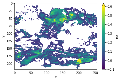
Diagnostic Potential Predictability (DPP)

We can first use the [Resplandy 2015] and [Seferian 2018] method for computing DPP, by not “chunking”.

threshold = climpred.bootstrap.dpp_threshold(control3d,
                                             m=10,
                                             chunk=False,
                                             bootstrap=10)
DPP10 = climpred.stats.dpp(control3d, m=10, chunk=False)
DPP10.where(DPP10 > threshold).plot(yincrease=False, vmin=-0.1, vmax=0.6, cmap='viridis')

Now, we can turn on chunking (the default for this function) to use the [Boer 2004] method.

threshold = climpred.bootstrap.dpp_threshold(control3d,
                                             m=10,
                                             chunk=True,
                                             bootstrap=bootstrap)
DPP10 = climpred.stats.dpp(control3d, m=10, chunk=True)
DPP10.where(DPP10>0).plot(yincrease=False, vmin=-0.1, vmax=0.6, cmap='viridis')

<matplotlib.collections.QuadMesh at 0x123e8c208>

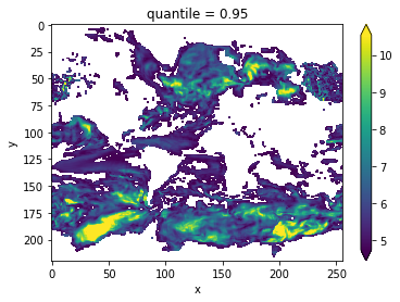
Variance-Weighted Mean Period

threshold = climpred.bootstrap.varweighted_mean_period_threshold(control3d,
                                                             bootstrap=bootstrap)
vwmp = climpred.stats.varweighted_mean_period(control3d, time_dim='time')
vwmp.where(vwmp > threshold).plot(yincrease=False, robust=True)

<matplotlib.collections.QuadMesh at 0x123ea8860>

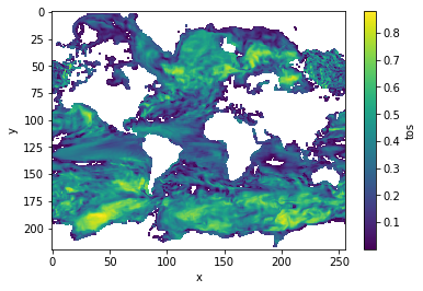
Lag-1 Autocorrelation

corr_ef = climpred.stats.autocorr(control3d, dim='time')
corr_ef.where(corr_ef>0).plot(yincrease=False, robust=False)

<matplotlib.collections.QuadMesh at 0x1c314b6860>

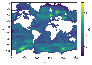
Decorrelation time

decorr_time = climpred.stats.decorrelation_time(control3d)
decorr_time.where(decorr_time>0).plot(yincrease=False, robust=False)

<matplotlib.collections.QuadMesh at 0x1c2e3a14a8>

References

1. Boer, Georges J. “Long time-scale potential predictability in an ensemble of coupled climate models.” Climate dynamics 23.1 (2004): 29-44.
2. Bushuk, Mitchell, Rym Msadek, Michael Winton, Gabriel Vecchi, Xiaosong Yang, Anthony Rosati, and Rich Gudgel. “Regional Arctic Sea–Ice Prediction: Potential versus Operational Seasonal Forecast Skill.” Climate Dynamics, June 9, 2018. https://doi.org/10/gd7hfq.
3. Collins, Matthew, and Sinha Bablu. “Predictability of Decadal Variations in the Thermohaline Circulation and Climate.” Geophysical Research Letters 30, no. 6 (March 22, 2003). https://doi.org/10/cts3cr.
4. Goddard, Lisa, et al. “A verification framework for interannual-to-decadal predictions experiments.” Climate Dynamics 40.1-2 (2013): 245-272.
5. Griffies, S. M., and K. Bryan. “A Predictability Study of Simulated North Atlantic Multidecadal Variability.” Climate Dynamics 13, no. 7–8 (August 1, 1997): 459–87. https://doi.org/10/ch4kc4.
6. Hawkins, Ed, Steffen Tietsche, Jonathan J. Day, Nathanael Melia, Keith Haines, and Sarah Keeley. “Aspects of Designing and Evaluating Seasonal-to-Interannual Arctic Sea-Ice Prediction Systems.” Quarterly Journal of the Royal Meteorological Society 142, no. 695 (January 1, 2016): 672–83. https://doi.org/10/gfb3pn.
7. Li, Hongmei, Tatiana Ilyina, Wolfgang A. Müller, and Frank Sienz. “Decadal Predictions of the North Atlantic CO2 Uptake.” Nature Communications 7 (March 30, 2016): 11076. https://doi.org/10/f8wkrs.
8. Pohlmann, Holger, Michael Botzet, Mojib Latif, Andreas Roesch, Martin Wild, and Peter Tschuck. “Estimating the Decadal Predictability of a Coupled AOGCM.” Journal of Climate 17, no. 22 (November 1, 2004): 4463–72. https://doi.org/10/d2qf62.
9. Resplandy, Laure, R. Séférian, and L. Bopp. “Natural variability of CO2 and O2 fluxes: What can we learn from centuries‐long climate models simulations?.” Journal of Geophysical Research: Oceans 120.1 (2015): 384-404.
10. Séférian, Roland, Sarah Berthet, and Matthieu Chevallier. “Assessing the Decadal Predictability of Land and Ocean Carbon Uptake.” Geophysical Research Letters, March 15, 2018. https://doi.org/10/gdb424.