Quick Start¶

The easiest way to get up and running is to load in one of our example datasets and to convert them to either a HindcastEnsemble or PerfectModelEnsemble object.

climpred provides various example datasets. See our examples to see some more analysis cases.

# linting
%load_ext nb_black
%load_ext lab_black

%matplotlib inline
import matplotlib.pyplot as plt
import xarray as xr

from climpred import HindcastEnsemble
from climpred.tutorial import load_dataset
import climpred

You can view the example datasets available to be loaded with climpred.tutorial.load_dataset() without passing any arguments:

load_dataset()

'MPI-control-1D': area averages for the MPI control run of SST/SSS.
'MPI-control-3D': lat/lon/time for the MPI control run of SST/SSS.
'MPI-PM-DP-1D': perfect model decadal prediction ensemble area averages of SST/SSS/AMO.
'MPI-PM-DP-3D': perfect model decadal prediction ensemble lat/lon/time of SST/SSS/AMO.
'CESM-DP-SST': hindcast decadal prediction ensemble of global mean SSTs.
'CESM-DP-SSS': hindcast decadal prediction ensemble of global mean SSS.
'CESM-DP-SST-3D': hindcast decadal prediction ensemble of eastern Pacific SSTs.
'CESM-LE': uninitialized ensemble of global mean SSTs.
'MPIESM_miklip_baseline1-hind-SST-global': hindcast initialized ensemble of global mean SSTs
'MPIESM_miklip_baseline1-hist-SST-global': uninitialized ensemble of global mean SSTs
'MPIESM_miklip_baseline1-assim-SST-global': assimilation in MPI-ESM of global mean SSTs
'ERSST': observations of global mean SSTs.
'FOSI-SST': reconstruction of global mean SSTs.
'FOSI-SSS': reconstruction of global mean SSS.
'FOSI-SST-3D': reconstruction of eastern Pacific SSTs
'GMAO-GEOS-RMM1': daily RMM1 from the GMAO-GEOS-V2p1 model for SubX
'RMM-INTERANN-OBS': observed RMM with interannual variablity included
'ECMWF_S2S_Germany': S2S ECMWF on-the-fly hindcasts from the S2S Project for Germany
'Observations_Germany': CPC/ERA5 observations for S2S forecasts over Germany
'NMME_hindcast_Nino34_sst': monthly multi-member hindcasts of sea-surface temperature averaged over the Nino3.4 region from the NMME project from IRIDL
'NMME_OIv2_Nino34_sst': monthly Reyn_SmithOIv2 sea-surface temperature observations averaged over the Nino3.4 region

From here, loading a dataset is easy. Note that you need to be connected to the internet for this to work – the datasets are being pulled from the climpred-data repository. Once loaded, it is cached on your computer so you can reload extremely quickly. These datasets are very small (< 1MB each) so they won’t take up much space.

initialized = climpred.tutorial.load_dataset("CESM-DP-SST")
# Add lead attribute units.
initialized["lead"].attrs["units"] = "years"
obs = climpred.tutorial.load_dataset("ERSST")

Make sure your prediction ensemble’s dimension labeling conforms to climpred’s standards. In other words, you need an init, lead, and (optional) member dimension. Make sure that your init and lead dimensions align.

Note that we here have a special case with ints in the init coords. For CESM-DP, a November 1st 1954 initialization should be labeled as init=1954, so that the lead=1 forecast related to valid_time=1955.

initialized.coords

Coordinates:
  * lead     (lead) int32 1 2 3 4 5 6 7 8 9 10
  * member   (member) int32 1 2 3 4 5 6 7 8 9 10
  * init     (init) float32 1.954e+03 1.955e+03 ... 2.016e+03 2.017e+03

We’ll quickly process the data to create anomalies. CESM-DPLE’s drift-correction occurs over 1964-2014, so we’ll remove that from the observations.

obs = obs - obs.sel(time=slice(1964, 2014)).mean("time")

We can create a HindcastEnsemble object and add our observations.

In forecast verification, valid_time for the initialized data shall be matched with time for observations.

hindcast.get_initialized().coords

Coordinates:
  * lead        (lead) int32 1 2 3 4 5 6 7 8 9 10
  * member      (member) int32 1 2 3 4 5 6 7 8 9 10
  * init        (init) object 1954-01-01 00:00:00 ... 2017-01-01 00:00:00
    valid_time  (lead, init) object 1955-01-01 00:00:00 ... 2027-01-01 00:00:00

hindcast.get_observations().coords

Coordinates:
  * time     (time) object 1955-01-01 00:00:00 ... 2015-01-01 00:00:00

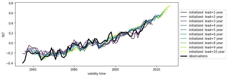
PredictionEnsemble.plot() shows all associated datasets (initialized, uninitialized if present, observations if present) if only climpred dimension (lead, init, member, time) are present, e.g. plot() does not work for lat, lon, model, …

hindcast.plot()

<AxesSubplot:xlabel='validity time', ylabel='SST'>

We’ll also remove a quadratic trend so that it doesn’t artificially boost our predictability. PredictionEnsemble.map(func) tries to apply/map a callable func to all associated datasets. Those calls do not raise errors such as ValueError, KeyError, DimensionError, but show respective warnings, which can be filtered away with warnings.filterwarnings("ignore").

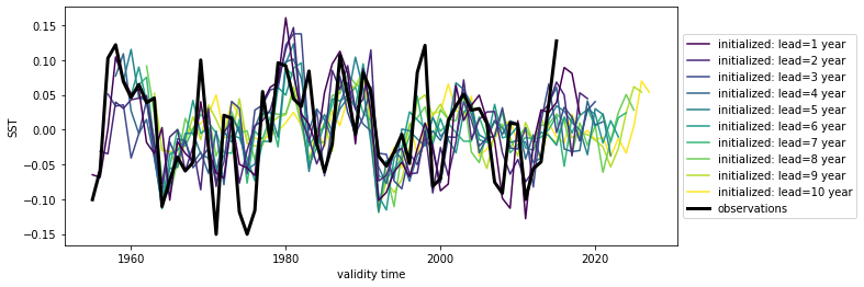
Alternatively, when supplying the kwargs dim="init_or_time", the matching dim is applied only and hence does not raise UserWarnings.

hindcast = hindcast.map(rm_poly, dim="init_or_time", deg=2)
hindcast.plot()

<AxesSubplot:xlabel='validity time', ylabel='SST'>

Now we’ll quickly calculate forecast with HindcastEnsemble.verify(). We require users to define metric, comparison, dim, and alignment. This ensures that climpred isn’t treated like a black box – there are no “defaults” to the prediction analysis framework. You can choose from a variety of possible metrics by entering their associated strings. comparisons strategies vary for hindcast and perfect model systems. Here we chose to compare the ensemble mean to observations ("e2o"). We reduce this operation over the initialization dimension. Lastly, we choose the "same_verif" alignment, which uses the same set of verification dates across all leads, see alignment strategies.

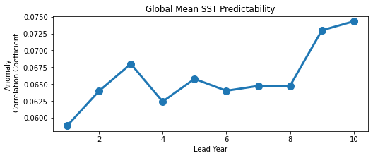
plt.rcParams["lines.linewidth"] = 3
plt.rcParams["lines.markersize"] = 10
plt.rcParams["lines.marker"] = "o"
plt.rcParams["figure.figsize"] = (8, 3)

result.SST.plot()
plt.title("Global Mean SST Predictability")
plt.ylabel("Anomaly \n Correlation Coefficient")
plt.xlabel("Lead Year")
plt.show()

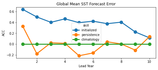
We can also check the association of forecasts and observations with the anomaly correlation coefficient metric="acc" climpred.metrics._pearson_r() against multiple reference forecasts. Choose reference from ["climatology","persistence","uninitialized"].

result = hindcast.verify(
    metric="acc",
    comparison="e2o",
    dim="init",
    alignment="same_verif",
    reference=["persistence", "climatology"],
)

result.SST.plot(hue="skill")
plt.title("Global Mean SST Forecast Error")
plt.ylabel("ACC")
plt.xlabel("Lead Year")
plt.show()

climpred documentation

Quick Start¶

climpred.HindcastEnsemble

climpred.HindcastEnsemble