You can run this notebook in a live session ![]() or view it on Github.
or view it on Github.
PredictionEnsemble Objects
One of the major features of climpred is our objects that are based upon the PredictionEnsemble class. We supply users with a HindcastEnsemble or PerfectModelEnsemble object. We encourage users to take advantage of these high-level objects, which wrap all of our core functions.
Briefly, we consider a HindcastEnsemble to be one that is initialized from some observational-like product (e.g., assimilated data, reanalysis products, or a model reconstruction). Thus, this object is built around comparing the initialized ensemble to various observational products.
In contrast, a PerfectModelEnsemble is one that is initialized off of a model control simulation. These forecasting systems are not meant to be compared directly to real-world observations. Instead, they provide a contained model environment with which to theoretically study the limits of predictability. You can read more about the terminology used in climpred here.
Let’s create a demo object to explore some of the functionality and why they are much smoother to use than direct function calls.
# linting
%load_ext nb_black
%load_ext lab_black
%matplotlib inline
import matplotlib.pyplot as plt
import xarray as xr
import numpy as np

from climpred import HindcastEnsemble, PerfectModelEnsemble
from climpred.tutorial import load_dataset
import climpred
We can now pull in some sample data that is packaged with climpred. We’ll start out with a HindcastEnsemble demo, followed by a PerfectModelEnsemble case.
HindcastEnsemble
initialized = climpred.tutorial.load_dataset(
    "CESM-DP-SST"
)  # CESM-DPLE hindcast ensemble output.
obs = climpred.tutorial.load_dataset("ERSST")  # ERSST observations.
We need to add a units attribute to the hindcast ensemble so that climpred knows how to interpret the lead units.
initialized["lead"].attrs["units"] = "years"
Now we instantiate the HindcastEnsemble object and append all of our products to it.
hindcast = HindcastEnsemble(
    initialized
)  # Instantiate object by passing in our initialized ensemble.
hindcast
/Users/aaron.spring/Coding/climpred/climpred/utils.py:191: UserWarning: Assuming annual resolution starting Jan 1st due to numeric inits. Please change ``init`` to a datetime if it is another resolution. We recommend using xr.CFTimeIndex as ``init``, see https://climpred.readthedocs.io/en/stable/setting-up-data.html.
  warnings.warn(
climpred.HindcastEnsemble
<Initialized Ensemble>
Dimensions:     (lead: 10, member: 10, init: 64)
Coordinates:
  * lead        (lead) int32 1 2 3 4 5 6 7 8 9 10
  * member      (member) int32 1 2 3 4 5 6 7 8 9 10
  * init        (init) object 1954-01-01 00:00:00 ... 2017-01-01 00:00:00
    valid_time  (lead, init) object 1955-01-01 00:00:00 ... 2027-01-01 00:00:00
Data variables:
SST (init, lead, member) float64 -0.2404 -0.2085 ... 0.7442 0.7384- lead: 10
- member: 10
- init: 64
- lead(lead)int321 2 3 4 5 6 7 8 9 10
- long_name :
- Lead
- units :
- years
- standard_name :
- forecast_period
- description :
- Forecast period is the time interval between the forecast reference time and the validity time. A period is an interval of time, or the time-period of an oscillation.
array([ 1, 2, 3, 4, 5, 6, 7, 8, 9, 10], dtype=int32)
- member(member)int321 2 3 4 5 6 7 8 9 10
- long_name :
- Member
- standard_name :
- realization
- description :
- Realization is used to label a dimension that can be thought of as a statistical sample, e.g., labelling members of a model ensemble.
array([ 1, 2, 3, 4, 5, 6, 7, 8, 9, 10], dtype=int32)
- init(init)object1954-01-01 00:00:00 ... 2017-01-...
- standard_name :
- forecast_reference_time
- long_name :
- Initialization
- description :
- The forecast reference time in NWP is the "data time", the time of the analysis from which the forecast was made. It is not the time for which the forecast is valid; the standard name of time should be used for that time.
array([cftime.DatetimeProlepticGregorian(1954, 1, 1, 0, 0, 0, 0, has_year_zero=True), cftime.DatetimeProlepticGregorian(1955, 1, 1, 0, 0, 0, 0, has_year_zero=True), cftime.DatetimeProlepticGregorian(1956, 1, 1, 0, 0, 0, 0, has_year_zero=True), cftime.DatetimeProlepticGregorian(1957, 1, 1, 0, 0, 0, 0, has_year_zero=True), cftime.DatetimeProlepticGregorian(1958, 1, 1, 0, 0, 0, 0, has_year_zero=True), cftime.DatetimeProlepticGregorian(1959, 1, 1, 0, 0, 0, 0, has_year_zero=True), cftime.DatetimeProlepticGregorian(1960, 1, 1, 0, 0, 0, 0, has_year_zero=True), cftime.DatetimeProlepticGregorian(1961, 1, 1, 0, 0, 0, 0, has_year_zero=True), cftime.DatetimeProlepticGregorian(1962, 1, 1, 0, 0, 0, 0, has_year_zero=True), cftime.DatetimeProlepticGregorian(1963, 1, 1, 0, 0, 0, 0, has_year_zero=True), cftime.DatetimeProlepticGregorian(1964, 1, 1, 0, 0, 0, 0, has_year_zero=True), cftime.DatetimeProlepticGregorian(1965, 1, 1, 0, 0, 0, 0, has_year_zero=True), cftime.DatetimeProlepticGregorian(1966, 1, 1, 0, 0, 0, 0, has_year_zero=True), cftime.DatetimeProlepticGregorian(1967, 1, 1, 0, 0, 0, 0, has_year_zero=True), cftime.DatetimeProlepticGregorian(1968, 1, 1, 0, 0, 0, 0, has_year_zero=True), cftime.DatetimeProlepticGregorian(1969, 1, 1, 0, 0, 0, 0, has_year_zero=True), cftime.DatetimeProlepticGregorian(1970, 1, 1, 0, 0, 0, 0, has_year_zero=True), cftime.DatetimeProlepticGregorian(1971, 1, 1, 0, 0, 0, 0, has_year_zero=True), cftime.DatetimeProlepticGregorian(1972, 1, 1, 0, 0, 0, 0, has_year_zero=True), cftime.DatetimeProlepticGregorian(1973, 1, 1, 0, 0, 0, 0, has_year_zero=True), cftime.DatetimeProlepticGregorian(1974, 1, 1, 0, 0, 0, 0, has_year_zero=True), cftime.DatetimeProlepticGregorian(1975, 1, 1, 0, 0, 0, 0, has_year_zero=True), cftime.DatetimeProlepticGregorian(1976, 1, 1, 0, 0, 0, 0, has_year_zero=True), cftime.DatetimeProlepticGregorian(1977, 1, 1, 0, 0, 0, 0, has_year_zero=True), cftime.DatetimeProlepticGregorian(1978, 1, 1, 0, 0, 0, 0, has_year_zero=True), cftime.DatetimeProlepticGregorian(1979, 1, 1, 0, 0, 0, 0, has_year_zero=True), cftime.DatetimeProlepticGregorian(1980, 1, 1, 0, 0, 0, 0, has_year_zero=True), cftime.DatetimeProlepticGregorian(1981, 1, 1, 0, 0, 0, 0, has_year_zero=True), cftime.DatetimeProlepticGregorian(1982, 1, 1, 0, 0, 0, 0, has_year_zero=True), cftime.DatetimeProlepticGregorian(1983, 1, 1, 0, 0, 0, 0, has_year_zero=True), cftime.DatetimeProlepticGregorian(1984, 1, 1, 0, 0, 0, 0, has_year_zero=True), cftime.DatetimeProlepticGregorian(1985, 1, 1, 0, 0, 0, 0, has_year_zero=True), cftime.DatetimeProlepticGregorian(1986, 1, 1, 0, 0, 0, 0, has_year_zero=True), cftime.DatetimeProlepticGregorian(1987, 1, 1, 0, 0, 0, 0, has_year_zero=True), cftime.DatetimeProlepticGregorian(1988, 1, 1, 0, 0, 0, 0, has_year_zero=True), cftime.DatetimeProlepticGregorian(1989, 1, 1, 0, 0, 0, 0, has_year_zero=True), cftime.DatetimeProlepticGregorian(1990, 1, 1, 0, 0, 0, 0, has_year_zero=True), cftime.DatetimeProlepticGregorian(1991, 1, 1, 0, 0, 0, 0, has_year_zero=True), cftime.DatetimeProlepticGregorian(1992, 1, 1, 0, 0, 0, 0, has_year_zero=True), cftime.DatetimeProlepticGregorian(1993, 1, 1, 0, 0, 0, 0, has_year_zero=True), cftime.DatetimeProlepticGregorian(1994, 1, 1, 0, 0, 0, 0, has_year_zero=True), cftime.DatetimeProlepticGregorian(1995, 1, 1, 0, 0, 0, 0, has_year_zero=True), cftime.DatetimeProlepticGregorian(1996, 1, 1, 0, 0, 0, 0, has_year_zero=True), cftime.DatetimeProlepticGregorian(1997, 1, 1, 0, 0, 0, 0, has_year_zero=True), cftime.DatetimeProlepticGregorian(1998, 1, 1, 0, 0, 0, 0, has_year_zero=True), cftime.DatetimeProlepticGregorian(1999, 1, 1, 0, 0, 0, 0, has_year_zero=True), cftime.DatetimeProlepticGregorian(2000, 1, 1, 0, 0, 0, 0, has_year_zero=True), cftime.DatetimeProlepticGregorian(2001, 1, 1, 0, 0, 0, 0, has_year_zero=True), cftime.DatetimeProlepticGregorian(2002, 1, 1, 0, 0, 0, 0, has_year_zero=True), cftime.DatetimeProlepticGregorian(2003, 1, 1, 0, 0, 0, 0, has_year_zero=True), cftime.DatetimeProlepticGregorian(2004, 1, 1, 0, 0, 0, 0, has_year_zero=True), cftime.DatetimeProlepticGregorian(2005, 1, 1, 0, 0, 0, 0, has_year_zero=True), cftime.DatetimeProlepticGregorian(2006, 1, 1, 0, 0, 0, 0, has_year_zero=True), cftime.DatetimeProlepticGregorian(2007, 1, 1, 0, 0, 0, 0, has_year_zero=True), cftime.DatetimeProlepticGregorian(2008, 1, 1, 0, 0, 0, 0, has_year_zero=True), cftime.DatetimeProlepticGregorian(2009, 1, 1, 0, 0, 0, 0, has_year_zero=True), cftime.DatetimeProlepticGregorian(2010, 1, 1, 0, 0, 0, 0, has_year_zero=True), cftime.DatetimeProlepticGregorian(2011, 1, 1, 0, 0, 0, 0, has_year_zero=True), cftime.DatetimeProlepticGregorian(2012, 1, 1, 0, 0, 0, 0, has_year_zero=True), cftime.DatetimeProlepticGregorian(2013, 1, 1, 0, 0, 0, 0, has_year_zero=True), cftime.DatetimeProlepticGregorian(2014, 1, 1, 0, 0, 0, 0, has_year_zero=True), cftime.DatetimeProlepticGregorian(2015, 1, 1, 0, 0, 0, 0, has_year_zero=True), cftime.DatetimeProlepticGregorian(2016, 1, 1, 0, 0, 0, 0, has_year_zero=True), cftime.DatetimeProlepticGregorian(2017, 1, 1, 0, 0, 0, 0, has_year_zero=True)], dtype=object) - valid_time(lead, init)object1955-01-01 00:00:00 ... 2027-01-...
- long_name :
- validity time
- standard_name :
- time
- description :
- time for which the forecast is valid
- calculate :
- init + lead
- amip :
- time
array([[cftime.DatetimeProlepticGregorian(1955, 1, 1, 0, 0, 0, 0, has_year_zero=True),
        cftime.DatetimeProlepticGregorian(1956, 1, 1, 0, 0, 0, 0, has_year_zero=True),
        cftime.DatetimeProlepticGregorian(1957, 1, 1, 0, 0, 0, 0, has_year_zero=True),
        cftime.DatetimeProlepticGregorian(1958, 1, 1, 0, 0, 0, 0, has_year_zero=True),
        cftime.DatetimeProlepticGregorian(1959, 1, 1, 0, 0, 0, 0, has_year_zero=True),
        cftime.DatetimeProlepticGregorian(1960, 1, 1, 0, 0, 0, 0, has_year_zero=True),
        cftime.DatetimeProlepticGregorian(1961, 1, 1, 0, 0, 0, 0, has_year_zero=True),
        cftime.DatetimeProlepticGregorian(1962, 1, 1, 0, 0, 0, 0, has_year_zero=True),
        cftime.DatetimeProlepticGregorian(1963, 1, 1, 0, 0, 0, 0, has_year_zero=True),
        cftime.DatetimeProlepticGregorian(1964, 1, 1, 0, 0, 0, 0, has_year_zero=True),
        cftime.DatetimeProlepticGregorian(1965, 1, 1, 0, 0, 0, 0, has_year_zero=True),
        cftime.DatetimeProlepticGregorian(1966, 1, 1, 0, 0, 0, 0, has_year_zero=True),
        cftime.DatetimeProlepticGregorian(1967, 1, 1, 0, 0, 0, 0, has_year_zero=True),
        cftime.DatetimeProlepticGregorian(1968, 1, 1, 0, 0, 0, 0, has_year_zero=True),
        cftime.DatetimeProlepticGregorian(1969, 1, 1, 0, 0, 0, 0, has_year_zero=True),
        cftime.DatetimeProlepticGregorian(1970, 1, 1, 0, 0, 0, 0, has_year_zero=True),
        cftime.DatetimeProlepticGregorian(1971, 1, 1, 0, 0, 0, 0, has_year_zero=True),
        cftime.DatetimeProlepticGregorian(1972, 1, 1, 0, 0, 0, 0, has_year_zero=True),
        cftime.DatetimeProlepticGregorian(1973, 1, 1, 0, 0, 0, 0, has_year_zero=True),
        cftime.DatetimeProlepticGregorian(1974, 1, 1, 0, 0, 0, 0, has_year_zero=True),
...
        cftime.DatetimeProlepticGregorian(2009, 1, 1, 0, 0, 0, 0, has_year_zero=True),
        cftime.DatetimeProlepticGregorian(2010, 1, 1, 0, 0, 0, 0, has_year_zero=True),
        cftime.DatetimeProlepticGregorian(2011, 1, 1, 0, 0, 0, 0, has_year_zero=True),
        cftime.DatetimeProlepticGregorian(2012, 1, 1, 0, 0, 0, 0, has_year_zero=True),
        cftime.DatetimeProlepticGregorian(2013, 1, 1, 0, 0, 0, 0, has_year_zero=True),
        cftime.DatetimeProlepticGregorian(2014, 1, 1, 0, 0, 0, 0, has_year_zero=True),
        cftime.DatetimeProlepticGregorian(2015, 1, 1, 0, 0, 0, 0, has_year_zero=True),
        cftime.DatetimeProlepticGregorian(2016, 1, 1, 0, 0, 0, 0, has_year_zero=True),
        cftime.DatetimeProlepticGregorian(2017, 1, 1, 0, 0, 0, 0, has_year_zero=True),
        cftime.DatetimeProlepticGregorian(2018, 1, 1, 0, 0, 0, 0, has_year_zero=True),
        cftime.DatetimeProlepticGregorian(2019, 1, 1, 0, 0, 0, 0, has_year_zero=True),
        cftime.DatetimeProlepticGregorian(2020, 1, 1, 0, 0, 0, 0, has_year_zero=True),
        cftime.DatetimeProlepticGregorian(2021, 1, 1, 0, 0, 0, 0, has_year_zero=True),
        cftime.DatetimeProlepticGregorian(2022, 1, 1, 0, 0, 0, 0, has_year_zero=True),
        cftime.DatetimeProlepticGregorian(2023, 1, 1, 0, 0, 0, 0, has_year_zero=True),
        cftime.DatetimeProlepticGregorian(2024, 1, 1, 0, 0, 0, 0, has_year_zero=True),
        cftime.DatetimeProlepticGregorian(2025, 1, 1, 0, 0, 0, 0, has_year_zero=True),
        cftime.DatetimeProlepticGregorian(2026, 1, 1, 0, 0, 0, 0, has_year_zero=True),
        cftime.DatetimeProlepticGregorian(2027, 1, 1, 0, 0, 0, 0, has_year_zero=True)]],
      dtype=object)
- SST(init, lead, member)float64-0.2404 -0.2085 ... 0.7442 0.7384
array([[[-0.240413, -0.208457, ..., -0.213875, -0.258075],
        [-0.156016, -0.145072, ..., -0.107661, -0.218739],
        ...,
        [-0.177814, -0.265736, ..., -0.233426, -0.111598],
        [-0.272566, -0.254668, ..., -0.290319, -0.262668]],

       [[-0.229101, -0.249644, ..., -0.208749, -0.215801],
        [-0.221161, -0.161461, ..., -0.121801, -0.178777],
        ...,
        [-0.255896, -0.278215, ..., -0.341992, -0.300791],
        [-0.270394, -0.243742, ..., -0.309798, -0.269629]],

       ...,

       [[ 0.376788,  0.39756 , ...,  0.462126,  0.433093],
        [ 0.532646,  0.469152, ...,  0.566459,  0.411788],
        ...,
        [ 0.728877,  0.737079, ...,  0.661647,  0.769273],
        [ 0.818281,  0.707076, ...,  0.751508,  0.86192 ]],

       [[ 0.37957 ,  0.41185 , ...,  0.363099,  0.391315],
        [ 0.47628 ,  0.614663, ...,  0.494712,  0.51935 ],
        ...,
        [ 0.742388,  0.69014 , ...,  0.786639,  0.771886],
        [ 0.77069 ,  0.747703, ...,  0.74417 ,  0.738442]]])
Now we just use HindcastEnsemble.add_observations() to attach other objects. See the API here. Note that we strive to make our conventions follow those of xarray. For example, we don’t allow inplace operations. One has to run hindcast = hindcast.add_observations(...) to modify the object upon later calls rather than just hindcast.add_observations(...).
hindcast = hindcast.add_observations(obs)
hindcast
/Users/aaron.spring/Coding/climpred/climpred/utils.py:191: UserWarning: Assuming annual resolution starting Jan 1st due to numeric inits. Please change ``init`` to a datetime if it is another resolution. We recommend using xr.CFTimeIndex as ``init``, see https://climpred.readthedocs.io/en/stable/setting-up-data.html.
  warnings.warn(
climpred.HindcastEnsemble
<Initialized Ensemble>
Dimensions:     (lead: 10, member: 10, init: 64)
Coordinates:
  * lead        (lead) int32 1 2 3 4 5 6 7 8 9 10
  * member      (member) int32 1 2 3 4 5 6 7 8 9 10
  * init        (init) object 1954-01-01 00:00:00 ... 2017-01-01 00:00:00
    valid_time  (lead, init) object 1955-01-01 00:00:00 ... 2027-01-01 00:00:00
Data variables:
SST (init, lead, member) float64 -0.2404 -0.2085 ... 0.7442 0.7384- lead: 10
- member: 10
- init: 64
- lead(lead)int321 2 3 4 5 6 7 8 9 10
- long_name :
- Lead
- units :
- years
- standard_name :
- forecast_period
- description :
- Forecast period is the time interval between the forecast reference time and the validity time. A period is an interval of time, or the time-period of an oscillation.
array([ 1, 2, 3, 4, 5, 6, 7, 8, 9, 10], dtype=int32)
- member(member)int321 2 3 4 5 6 7 8 9 10
- long_name :
- Member
- standard_name :
- realization
- description :
- Realization is used to label a dimension that can be thought of as a statistical sample, e.g., labelling members of a model ensemble.
array([ 1, 2, 3, 4, 5, 6, 7, 8, 9, 10], dtype=int32)
- init(init)object1954-01-01 00:00:00 ... 2017-01-...
- standard_name :
- forecast_reference_time
- long_name :
- Initialization
- description :
- The forecast reference time in NWP is the "data time", the time of the analysis from which the forecast was made. It is not the time for which the forecast is valid; the standard name of time should be used for that time.
array([cftime.DatetimeProlepticGregorian(1954, 1, 1, 0, 0, 0, 0, has_year_zero=True), cftime.DatetimeProlepticGregorian(1955, 1, 1, 0, 0, 0, 0, has_year_zero=True), cftime.DatetimeProlepticGregorian(1956, 1, 1, 0, 0, 0, 0, has_year_zero=True), cftime.DatetimeProlepticGregorian(1957, 1, 1, 0, 0, 0, 0, has_year_zero=True), cftime.DatetimeProlepticGregorian(1958, 1, 1, 0, 0, 0, 0, has_year_zero=True), cftime.DatetimeProlepticGregorian(1959, 1, 1, 0, 0, 0, 0, has_year_zero=True), cftime.DatetimeProlepticGregorian(1960, 1, 1, 0, 0, 0, 0, has_year_zero=True), cftime.DatetimeProlepticGregorian(1961, 1, 1, 0, 0, 0, 0, has_year_zero=True), cftime.DatetimeProlepticGregorian(1962, 1, 1, 0, 0, 0, 0, has_year_zero=True), cftime.DatetimeProlepticGregorian(1963, 1, 1, 0, 0, 0, 0, has_year_zero=True), cftime.DatetimeProlepticGregorian(1964, 1, 1, 0, 0, 0, 0, has_year_zero=True), cftime.DatetimeProlepticGregorian(1965, 1, 1, 0, 0, 0, 0, has_year_zero=True), cftime.DatetimeProlepticGregorian(1966, 1, 1, 0, 0, 0, 0, has_year_zero=True), cftime.DatetimeProlepticGregorian(1967, 1, 1, 0, 0, 0, 0, has_year_zero=True), cftime.DatetimeProlepticGregorian(1968, 1, 1, 0, 0, 0, 0, has_year_zero=True), cftime.DatetimeProlepticGregorian(1969, 1, 1, 0, 0, 0, 0, has_year_zero=True), cftime.DatetimeProlepticGregorian(1970, 1, 1, 0, 0, 0, 0, has_year_zero=True), cftime.DatetimeProlepticGregorian(1971, 1, 1, 0, 0, 0, 0, has_year_zero=True), cftime.DatetimeProlepticGregorian(1972, 1, 1, 0, 0, 0, 0, has_year_zero=True), cftime.DatetimeProlepticGregorian(1973, 1, 1, 0, 0, 0, 0, has_year_zero=True), cftime.DatetimeProlepticGregorian(1974, 1, 1, 0, 0, 0, 0, has_year_zero=True), cftime.DatetimeProlepticGregorian(1975, 1, 1, 0, 0, 0, 0, has_year_zero=True), cftime.DatetimeProlepticGregorian(1976, 1, 1, 0, 0, 0, 0, has_year_zero=True), cftime.DatetimeProlepticGregorian(1977, 1, 1, 0, 0, 0, 0, has_year_zero=True), cftime.DatetimeProlepticGregorian(1978, 1, 1, 0, 0, 0, 0, has_year_zero=True), cftime.DatetimeProlepticGregorian(1979, 1, 1, 0, 0, 0, 0, has_year_zero=True), cftime.DatetimeProlepticGregorian(1980, 1, 1, 0, 0, 0, 0, has_year_zero=True), cftime.DatetimeProlepticGregorian(1981, 1, 1, 0, 0, 0, 0, has_year_zero=True), cftime.DatetimeProlepticGregorian(1982, 1, 1, 0, 0, 0, 0, has_year_zero=True), cftime.DatetimeProlepticGregorian(1983, 1, 1, 0, 0, 0, 0, has_year_zero=True), cftime.DatetimeProlepticGregorian(1984, 1, 1, 0, 0, 0, 0, has_year_zero=True), cftime.DatetimeProlepticGregorian(1985, 1, 1, 0, 0, 0, 0, has_year_zero=True), cftime.DatetimeProlepticGregorian(1986, 1, 1, 0, 0, 0, 0, has_year_zero=True), cftime.DatetimeProlepticGregorian(1987, 1, 1, 0, 0, 0, 0, has_year_zero=True), cftime.DatetimeProlepticGregorian(1988, 1, 1, 0, 0, 0, 0, has_year_zero=True), cftime.DatetimeProlepticGregorian(1989, 1, 1, 0, 0, 0, 0, has_year_zero=True), cftime.DatetimeProlepticGregorian(1990, 1, 1, 0, 0, 0, 0, has_year_zero=True), cftime.DatetimeProlepticGregorian(1991, 1, 1, 0, 0, 0, 0, has_year_zero=True), cftime.DatetimeProlepticGregorian(1992, 1, 1, 0, 0, 0, 0, has_year_zero=True), cftime.DatetimeProlepticGregorian(1993, 1, 1, 0, 0, 0, 0, has_year_zero=True), cftime.DatetimeProlepticGregorian(1994, 1, 1, 0, 0, 0, 0, has_year_zero=True), cftime.DatetimeProlepticGregorian(1995, 1, 1, 0, 0, 0, 0, has_year_zero=True), cftime.DatetimeProlepticGregorian(1996, 1, 1, 0, 0, 0, 0, has_year_zero=True), cftime.DatetimeProlepticGregorian(1997, 1, 1, 0, 0, 0, 0, has_year_zero=True), cftime.DatetimeProlepticGregorian(1998, 1, 1, 0, 0, 0, 0, has_year_zero=True), cftime.DatetimeProlepticGregorian(1999, 1, 1, 0, 0, 0, 0, has_year_zero=True), cftime.DatetimeProlepticGregorian(2000, 1, 1, 0, 0, 0, 0, has_year_zero=True), cftime.DatetimeProlepticGregorian(2001, 1, 1, 0, 0, 0, 0, has_year_zero=True), cftime.DatetimeProlepticGregorian(2002, 1, 1, 0, 0, 0, 0, has_year_zero=True), cftime.DatetimeProlepticGregorian(2003, 1, 1, 0, 0, 0, 0, has_year_zero=True), cftime.DatetimeProlepticGregorian(2004, 1, 1, 0, 0, 0, 0, has_year_zero=True), cftime.DatetimeProlepticGregorian(2005, 1, 1, 0, 0, 0, 0, has_year_zero=True), cftime.DatetimeProlepticGregorian(2006, 1, 1, 0, 0, 0, 0, has_year_zero=True), cftime.DatetimeProlepticGregorian(2007, 1, 1, 0, 0, 0, 0, has_year_zero=True), cftime.DatetimeProlepticGregorian(2008, 1, 1, 0, 0, 0, 0, has_year_zero=True), cftime.DatetimeProlepticGregorian(2009, 1, 1, 0, 0, 0, 0, has_year_zero=True), cftime.DatetimeProlepticGregorian(2010, 1, 1, 0, 0, 0, 0, has_year_zero=True), cftime.DatetimeProlepticGregorian(2011, 1, 1, 0, 0, 0, 0, has_year_zero=True), cftime.DatetimeProlepticGregorian(2012, 1, 1, 0, 0, 0, 0, has_year_zero=True), cftime.DatetimeProlepticGregorian(2013, 1, 1, 0, 0, 0, 0, has_year_zero=True), cftime.DatetimeProlepticGregorian(2014, 1, 1, 0, 0, 0, 0, has_year_zero=True), cftime.DatetimeProlepticGregorian(2015, 1, 1, 0, 0, 0, 0, has_year_zero=True), cftime.DatetimeProlepticGregorian(2016, 1, 1, 0, 0, 0, 0, has_year_zero=True), cftime.DatetimeProlepticGregorian(2017, 1, 1, 0, 0, 0, 0, has_year_zero=True)], dtype=object) - valid_time(lead, init)object1955-01-01 00:00:00 ... 2027-01-...
- long_name :
- validity time
- standard_name :
- time
- description :
- time for which the forecast is valid
- calculate :
- init + lead
- amip :
- time
array([[cftime.DatetimeProlepticGregorian(1955, 1, 1, 0, 0, 0, 0, has_year_zero=True),
        cftime.DatetimeProlepticGregorian(1956, 1, 1, 0, 0, 0, 0, has_year_zero=True),
        cftime.DatetimeProlepticGregorian(1957, 1, 1, 0, 0, 0, 0, has_year_zero=True),
        cftime.DatetimeProlepticGregorian(1958, 1, 1, 0, 0, 0, 0, has_year_zero=True),
        cftime.DatetimeProlepticGregorian(1959, 1, 1, 0, 0, 0, 0, has_year_zero=True),
        cftime.DatetimeProlepticGregorian(1960, 1, 1, 0, 0, 0, 0, has_year_zero=True),
        cftime.DatetimeProlepticGregorian(1961, 1, 1, 0, 0, 0, 0, has_year_zero=True),
        cftime.DatetimeProlepticGregorian(1962, 1, 1, 0, 0, 0, 0, has_year_zero=True),
        cftime.DatetimeProlepticGregorian(1963, 1, 1, 0, 0, 0, 0, has_year_zero=True),
        cftime.DatetimeProlepticGregorian(1964, 1, 1, 0, 0, 0, 0, has_year_zero=True),
        cftime.DatetimeProlepticGregorian(1965, 1, 1, 0, 0, 0, 0, has_year_zero=True),
        cftime.DatetimeProlepticGregorian(1966, 1, 1, 0, 0, 0, 0, has_year_zero=True),
        cftime.DatetimeProlepticGregorian(1967, 1, 1, 0, 0, 0, 0, has_year_zero=True),
        cftime.DatetimeProlepticGregorian(1968, 1, 1, 0, 0, 0, 0, has_year_zero=True),
        cftime.DatetimeProlepticGregorian(1969, 1, 1, 0, 0, 0, 0, has_year_zero=True),
        cftime.DatetimeProlepticGregorian(1970, 1, 1, 0, 0, 0, 0, has_year_zero=True),
        cftime.DatetimeProlepticGregorian(1971, 1, 1, 0, 0, 0, 0, has_year_zero=True),
        cftime.DatetimeProlepticGregorian(1972, 1, 1, 0, 0, 0, 0, has_year_zero=True),
        cftime.DatetimeProlepticGregorian(1973, 1, 1, 0, 0, 0, 0, has_year_zero=True),
        cftime.DatetimeProlepticGregorian(1974, 1, 1, 0, 0, 0, 0, has_year_zero=True),
...
        cftime.DatetimeProlepticGregorian(2009, 1, 1, 0, 0, 0, 0, has_year_zero=True),
        cftime.DatetimeProlepticGregorian(2010, 1, 1, 0, 0, 0, 0, has_year_zero=True),
        cftime.DatetimeProlepticGregorian(2011, 1, 1, 0, 0, 0, 0, has_year_zero=True),
        cftime.DatetimeProlepticGregorian(2012, 1, 1, 0, 0, 0, 0, has_year_zero=True),
        cftime.DatetimeProlepticGregorian(2013, 1, 1, 0, 0, 0, 0, has_year_zero=True),
        cftime.DatetimeProlepticGregorian(2014, 1, 1, 0, 0, 0, 0, has_year_zero=True),
        cftime.DatetimeProlepticGregorian(2015, 1, 1, 0, 0, 0, 0, has_year_zero=True),
        cftime.DatetimeProlepticGregorian(2016, 1, 1, 0, 0, 0, 0, has_year_zero=True),
        cftime.DatetimeProlepticGregorian(2017, 1, 1, 0, 0, 0, 0, has_year_zero=True),
        cftime.DatetimeProlepticGregorian(2018, 1, 1, 0, 0, 0, 0, has_year_zero=True),
        cftime.DatetimeProlepticGregorian(2019, 1, 1, 0, 0, 0, 0, has_year_zero=True),
        cftime.DatetimeProlepticGregorian(2020, 1, 1, 0, 0, 0, 0, has_year_zero=True),
        cftime.DatetimeProlepticGregorian(2021, 1, 1, 0, 0, 0, 0, has_year_zero=True),
        cftime.DatetimeProlepticGregorian(2022, 1, 1, 0, 0, 0, 0, has_year_zero=True),
        cftime.DatetimeProlepticGregorian(2023, 1, 1, 0, 0, 0, 0, has_year_zero=True),
        cftime.DatetimeProlepticGregorian(2024, 1, 1, 0, 0, 0, 0, has_year_zero=True),
        cftime.DatetimeProlepticGregorian(2025, 1, 1, 0, 0, 0, 0, has_year_zero=True),
        cftime.DatetimeProlepticGregorian(2026, 1, 1, 0, 0, 0, 0, has_year_zero=True),
        cftime.DatetimeProlepticGregorian(2027, 1, 1, 0, 0, 0, 0, has_year_zero=True)]],
      dtype=object)
- SST(init, lead, member)float64-0.2404 -0.2085 ... 0.7442 0.7384
array([[[-0.240413, -0.208457, ..., -0.213875, -0.258075],
        [-0.156016, -0.145072, ..., -0.107661, -0.218739],
        ...,
        [-0.177814, -0.265736, ..., -0.233426, -0.111598],
        [-0.272566, -0.254668, ..., -0.290319, -0.262668]],

       [[-0.229101, -0.249644, ..., -0.208749, -0.215801],
        [-0.221161, -0.161461, ..., -0.121801, -0.178777],
        ...,
        [-0.255896, -0.278215, ..., -0.341992, -0.300791],
        [-0.270394, -0.243742, ..., -0.309798, -0.269629]],

       ...,

       [[ 0.376788,  0.39756 , ...,  0.462126,  0.433093],
        [ 0.532646,  0.469152, ...,  0.566459,  0.411788],
        ...,
        [ 0.728877,  0.737079, ...,  0.661647,  0.769273],
        [ 0.818281,  0.707076, ...,  0.751508,  0.86192 ]],

       [[ 0.37957 ,  0.41185 , ...,  0.363099,  0.391315],
        [ 0.47628 ,  0.614663, ...,  0.494712,  0.51935 ],
        ...,
        [ 0.742388,  0.69014 , ...,  0.786639,  0.771886],
        [ 0.77069 ,  0.747703, ...,  0.74417 ,  0.738442]]])
<Observations>
Dimensions:  (time: 61)
Coordinates:
  * time     (time) object 1955-01-01 00:00:00 ... 2015-01-01 00:00:00
Data variables:
SST (time) float32 17.79 17.84 18.0 18.03 ... 18.41 18.44 18.54 18.64- time: 61
- time(time)object1955-01-01 00:00:00 ... 2015-01-...
- long_name :
- time
- standard_name :
- time
array([cftime.DatetimeProlepticGregorian(1955, 1, 1, 0, 0, 0, 0, has_year_zero=True),
       cftime.DatetimeProlepticGregorian(1956, 1, 1, 0, 0, 0, 0, has_year_zero=True),
       cftime.DatetimeProlepticGregorian(1957, 1, 1, 0, 0, 0, 0, has_year_zero=True),
       cftime.DatetimeProlepticGregorian(1958, 1, 1, 0, 0, 0, 0, has_year_zero=True),
       cftime.DatetimeProlepticGregorian(1959, 1, 1, 0, 0, 0, 0, has_year_zero=True),
       cftime.DatetimeProlepticGregorian(1960, 1, 1, 0, 0, 0, 0, has_year_zero=True),
       cftime.DatetimeProlepticGregorian(1961, 1, 1, 0, 0, 0, 0, has_year_zero=True),
       cftime.DatetimeProlepticGregorian(1962, 1, 1, 0, 0, 0, 0, has_year_zero=True),
       cftime.DatetimeProlepticGregorian(1963, 1, 1, 0, 0, 0, 0, has_year_zero=True),
       cftime.DatetimeProlepticGregorian(1964, 1, 1, 0, 0, 0, 0, has_year_zero=True),
       cftime.DatetimeProlepticGregorian(1965, 1, 1, 0, 0, 0, 0, has_year_zero=True),
       cftime.DatetimeProlepticGregorian(1966, 1, 1, 0, 0, 0, 0, has_year_zero=True),
       cftime.DatetimeProlepticGregorian(1967, 1, 1, 0, 0, 0, 0, has_year_zero=True),
       cftime.DatetimeProlepticGregorian(1968, 1, 1, 0, 0, 0, 0, has_year_zero=True),
       cftime.DatetimeProlepticGregorian(1969, 1, 1, 0, 0, 0, 0, has_year_zero=True),
       cftime.DatetimeProlepticGregorian(1970, 1, 1, 0, 0, 0, 0, has_year_zero=True),
       cftime.DatetimeProlepticGregorian(1971, 1, 1, 0, 0, 0, 0, has_year_zero=True),
       cftime.DatetimeProlepticGregorian(1972, 1, 1, 0, 0, 0, 0, has_year_zero=True),
       cftime.DatetimeProlepticGregorian(1973, 1, 1, 0, 0, 0, 0, has_year_zero=True),
       cftime.DatetimeProlepticGregorian(1974, 1, 1, 0, 0, 0, 0, has_year_zero=True),
       cftime.DatetimeProlepticGregorian(1975, 1, 1, 0, 0, 0, 0, has_year_zero=True),
       cftime.DatetimeProlepticGregorian(1976, 1, 1, 0, 0, 0, 0, has_year_zero=True),
       cftime.DatetimeProlepticGregorian(1977, 1, 1, 0, 0, 0, 0, has_year_zero=True),
       cftime.DatetimeProlepticGregorian(1978, 1, 1, 0, 0, 0, 0, has_year_zero=True),
       cftime.DatetimeProlepticGregorian(1979, 1, 1, 0, 0, 0, 0, has_year_zero=True),
       cftime.DatetimeProlepticGregorian(1980, 1, 1, 0, 0, 0, 0, has_year_zero=True),
       cftime.DatetimeProlepticGregorian(1981, 1, 1, 0, 0, 0, 0, has_year_zero=True),
       cftime.DatetimeProlepticGregorian(1982, 1, 1, 0, 0, 0, 0, has_year_zero=True),
       cftime.DatetimeProlepticGregorian(1983, 1, 1, 0, 0, 0, 0, has_year_zero=True),
       cftime.DatetimeProlepticGregorian(1984, 1, 1, 0, 0, 0, 0, has_year_zero=True),
       cftime.DatetimeProlepticGregorian(1985, 1, 1, 0, 0, 0, 0, has_year_zero=True),
       cftime.DatetimeProlepticGregorian(1986, 1, 1, 0, 0, 0, 0, has_year_zero=True),
       cftime.DatetimeProlepticGregorian(1987, 1, 1, 0, 0, 0, 0, has_year_zero=True),
       cftime.DatetimeProlepticGregorian(1988, 1, 1, 0, 0, 0, 0, has_year_zero=True),
       cftime.DatetimeProlepticGregorian(1989, 1, 1, 0, 0, 0, 0, has_year_zero=True),
       cftime.DatetimeProlepticGregorian(1990, 1, 1, 0, 0, 0, 0, has_year_zero=True),
       cftime.DatetimeProlepticGregorian(1991, 1, 1, 0, 0, 0, 0, has_year_zero=True),
       cftime.DatetimeProlepticGregorian(1992, 1, 1, 0, 0, 0, 0, has_year_zero=True),
       cftime.DatetimeProlepticGregorian(1993, 1, 1, 0, 0, 0, 0, has_year_zero=True),
       cftime.DatetimeProlepticGregorian(1994, 1, 1, 0, 0, 0, 0, has_year_zero=True),
       cftime.DatetimeProlepticGregorian(1995, 1, 1, 0, 0, 0, 0, has_year_zero=True),
       cftime.DatetimeProlepticGregorian(1996, 1, 1, 0, 0, 0, 0, has_year_zero=True),
       cftime.DatetimeProlepticGregorian(1997, 1, 1, 0, 0, 0, 0, has_year_zero=True),
       cftime.DatetimeProlepticGregorian(1998, 1, 1, 0, 0, 0, 0, has_year_zero=True),
       cftime.DatetimeProlepticGregorian(1999, 1, 1, 0, 0, 0, 0, has_year_zero=True),
       cftime.DatetimeProlepticGregorian(2000, 1, 1, 0, 0, 0, 0, has_year_zero=True),
       cftime.DatetimeProlepticGregorian(2001, 1, 1, 0, 0, 0, 0, has_year_zero=True),
       cftime.DatetimeProlepticGregorian(2002, 1, 1, 0, 0, 0, 0, has_year_zero=True),
       cftime.DatetimeProlepticGregorian(2003, 1, 1, 0, 0, 0, 0, has_year_zero=True),
       cftime.DatetimeProlepticGregorian(2004, 1, 1, 0, 0, 0, 0, has_year_zero=True),
       cftime.DatetimeProlepticGregorian(2005, 1, 1, 0, 0, 0, 0, has_year_zero=True),
       cftime.DatetimeProlepticGregorian(2006, 1, 1, 0, 0, 0, 0, has_year_zero=True),
       cftime.DatetimeProlepticGregorian(2007, 1, 1, 0, 0, 0, 0, has_year_zero=True),
       cftime.DatetimeProlepticGregorian(2008, 1, 1, 0, 0, 0, 0, has_year_zero=True),
       cftime.DatetimeProlepticGregorian(2009, 1, 1, 0, 0, 0, 0, has_year_zero=True),
       cftime.DatetimeProlepticGregorian(2010, 1, 1, 0, 0, 0, 0, has_year_zero=True),
       cftime.DatetimeProlepticGregorian(2011, 1, 1, 0, 0, 0, 0, has_year_zero=True),
       cftime.DatetimeProlepticGregorian(2012, 1, 1, 0, 0, 0, 0, has_year_zero=True),
       cftime.DatetimeProlepticGregorian(2013, 1, 1, 0, 0, 0, 0, has_year_zero=True),
       cftime.DatetimeProlepticGregorian(2014, 1, 1, 0, 0, 0, 0, has_year_zero=True),
       cftime.DatetimeProlepticGregorian(2015, 1, 1, 0, 0, 0, 0, has_year_zero=True)],
      dtype=object)
- SST(time)float3217.79 17.84 18.0 ... 18.54 18.64
array([17.788563, 17.837637, 18.004938, 18.030924, 17.984966, 17.969116,
       17.995125, 17.976297, 17.990444, 17.842377, 17.888042, 17.928734,
       17.9168  , 17.937092, 18.092508, 17.977272, 17.859001, 18.038591,
       18.042986, 17.91727 , 17.894423, 17.937723, 18.117777, 18.055983,
       18.177963, 18.183275, 18.145844, 18.14466 , 18.205618, 18.112675,
       18.081434, 18.13182 , 18.269695, 18.223383, 18.178385, 18.277567,
       18.262365, 18.17984 , 18.177143, 18.208504, 18.245817, 18.215742,
       18.358284, 18.40929 , 18.219038, 18.24239 , 18.338306, 18.371956,
       18.401276, 18.391241, 18.406458, 18.39851 , 18.327087, 18.324453,
       18.438929, 18.450453, 18.356506, 18.414541, 18.438139, 18.536037,
       18.640236], dtype=float32)
You can apply most standard xarray functions directly to our objects! climpred will loop through the objects and apply the function to all applicable xarray.Dataset within the object. If you reference a dimension that doesn’t exist for the given xarray.Dataset, it will ignore it. This is useful, since the initialized ensemble is expected to have dimension init, while other products have dimension time (see more here).
Let’s start by taking the ensemble mean of the initialized ensemble. Just using deterministic metrics here, so we don’t need the individual ensemble members. Note that above our initialized ensemble had a member dimension, and now it is reduced. Those xarray functions do not raise errors such as ValueError, KeyError, DimensionError, but show respective warnings, which can be filtered away with warnings.filterwarnings("ignore").
hindcast = hindcast.mean("member")
hindcast
/Users/aaron.spring/Coding/climpred/climpred/classes.py:713: UserWarning: Error due to verification/control/uninitialized: xr.mean(('member',), {}) failed
ValueError: Dataset does not contain the dimensions: ['member']
  warnings.warn(
climpred.HindcastEnsemble
<Initialized Ensemble>
Dimensions:     (lead: 10, init: 64)
Coordinates:
  * lead        (lead) int32 1 2 3 4 5 6 7 8 9 10
  * init        (init) object 1954-01-01 00:00:00 ... 2017-01-01 00:00:00
    valid_time  (lead, init) object 1955-01-01 00:00:00 ... 2027-01-01 00:00:00
Data variables:
SST (init, lead) float64 -0.2121 -0.1637 -0.1206 ... 0.7286 0.7532- lead: 10
- init: 64
- lead(lead)int321 2 3 4 5 6 7 8 9 10
- long_name :
- Lead
- units :
- years
- standard_name :
- forecast_period
- description :
- Forecast period is the time interval between the forecast reference time and the validity time. A period is an interval of time, or the time-period of an oscillation.
array([ 1, 2, 3, 4, 5, 6, 7, 8, 9, 10], dtype=int32)
- init(init)object1954-01-01 00:00:00 ... 2017-01-...
- standard_name :
- forecast_reference_time
- long_name :
- Initialization
- description :
- The forecast reference time in NWP is the "data time", the time of the analysis from which the forecast was made. It is not the time for which the forecast is valid; the standard name of time should be used for that time.
array([cftime.DatetimeProlepticGregorian(1954, 1, 1, 0, 0, 0, 0, has_year_zero=True), cftime.DatetimeProlepticGregorian(1955, 1, 1, 0, 0, 0, 0, has_year_zero=True), cftime.DatetimeProlepticGregorian(1956, 1, 1, 0, 0, 0, 0, has_year_zero=True), cftime.DatetimeProlepticGregorian(1957, 1, 1, 0, 0, 0, 0, has_year_zero=True), cftime.DatetimeProlepticGregorian(1958, 1, 1, 0, 0, 0, 0, has_year_zero=True), cftime.DatetimeProlepticGregorian(1959, 1, 1, 0, 0, 0, 0, has_year_zero=True), cftime.DatetimeProlepticGregorian(1960, 1, 1, 0, 0, 0, 0, has_year_zero=True), cftime.DatetimeProlepticGregorian(1961, 1, 1, 0, 0, 0, 0, has_year_zero=True), cftime.DatetimeProlepticGregorian(1962, 1, 1, 0, 0, 0, 0, has_year_zero=True), cftime.DatetimeProlepticGregorian(1963, 1, 1, 0, 0, 0, 0, has_year_zero=True), cftime.DatetimeProlepticGregorian(1964, 1, 1, 0, 0, 0, 0, has_year_zero=True), cftime.DatetimeProlepticGregorian(1965, 1, 1, 0, 0, 0, 0, has_year_zero=True), cftime.DatetimeProlepticGregorian(1966, 1, 1, 0, 0, 0, 0, has_year_zero=True), cftime.DatetimeProlepticGregorian(1967, 1, 1, 0, 0, 0, 0, has_year_zero=True), cftime.DatetimeProlepticGregorian(1968, 1, 1, 0, 0, 0, 0, has_year_zero=True), cftime.DatetimeProlepticGregorian(1969, 1, 1, 0, 0, 0, 0, has_year_zero=True), cftime.DatetimeProlepticGregorian(1970, 1, 1, 0, 0, 0, 0, has_year_zero=True), cftime.DatetimeProlepticGregorian(1971, 1, 1, 0, 0, 0, 0, has_year_zero=True), cftime.DatetimeProlepticGregorian(1972, 1, 1, 0, 0, 0, 0, has_year_zero=True), cftime.DatetimeProlepticGregorian(1973, 1, 1, 0, 0, 0, 0, has_year_zero=True), cftime.DatetimeProlepticGregorian(1974, 1, 1, 0, 0, 0, 0, has_year_zero=True), cftime.DatetimeProlepticGregorian(1975, 1, 1, 0, 0, 0, 0, has_year_zero=True), cftime.DatetimeProlepticGregorian(1976, 1, 1, 0, 0, 0, 0, has_year_zero=True), cftime.DatetimeProlepticGregorian(1977, 1, 1, 0, 0, 0, 0, has_year_zero=True), cftime.DatetimeProlepticGregorian(1978, 1, 1, 0, 0, 0, 0, has_year_zero=True), cftime.DatetimeProlepticGregorian(1979, 1, 1, 0, 0, 0, 0, has_year_zero=True), cftime.DatetimeProlepticGregorian(1980, 1, 1, 0, 0, 0, 0, has_year_zero=True), cftime.DatetimeProlepticGregorian(1981, 1, 1, 0, 0, 0, 0, has_year_zero=True), cftime.DatetimeProlepticGregorian(1982, 1, 1, 0, 0, 0, 0, has_year_zero=True), cftime.DatetimeProlepticGregorian(1983, 1, 1, 0, 0, 0, 0, has_year_zero=True), cftime.DatetimeProlepticGregorian(1984, 1, 1, 0, 0, 0, 0, has_year_zero=True), cftime.DatetimeProlepticGregorian(1985, 1, 1, 0, 0, 0, 0, has_year_zero=True), cftime.DatetimeProlepticGregorian(1986, 1, 1, 0, 0, 0, 0, has_year_zero=True), cftime.DatetimeProlepticGregorian(1987, 1, 1, 0, 0, 0, 0, has_year_zero=True), cftime.DatetimeProlepticGregorian(1988, 1, 1, 0, 0, 0, 0, has_year_zero=True), cftime.DatetimeProlepticGregorian(1989, 1, 1, 0, 0, 0, 0, has_year_zero=True), cftime.DatetimeProlepticGregorian(1990, 1, 1, 0, 0, 0, 0, has_year_zero=True), cftime.DatetimeProlepticGregorian(1991, 1, 1, 0, 0, 0, 0, has_year_zero=True), cftime.DatetimeProlepticGregorian(1992, 1, 1, 0, 0, 0, 0, has_year_zero=True), cftime.DatetimeProlepticGregorian(1993, 1, 1, 0, 0, 0, 0, has_year_zero=True), cftime.DatetimeProlepticGregorian(1994, 1, 1, 0, 0, 0, 0, has_year_zero=True), cftime.DatetimeProlepticGregorian(1995, 1, 1, 0, 0, 0, 0, has_year_zero=True), cftime.DatetimeProlepticGregorian(1996, 1, 1, 0, 0, 0, 0, has_year_zero=True), cftime.DatetimeProlepticGregorian(1997, 1, 1, 0, 0, 0, 0, has_year_zero=True), cftime.DatetimeProlepticGregorian(1998, 1, 1, 0, 0, 0, 0, has_year_zero=True), cftime.DatetimeProlepticGregorian(1999, 1, 1, 0, 0, 0, 0, has_year_zero=True), cftime.DatetimeProlepticGregorian(2000, 1, 1, 0, 0, 0, 0, has_year_zero=True), cftime.DatetimeProlepticGregorian(2001, 1, 1, 0, 0, 0, 0, has_year_zero=True), cftime.DatetimeProlepticGregorian(2002, 1, 1, 0, 0, 0, 0, has_year_zero=True), cftime.DatetimeProlepticGregorian(2003, 1, 1, 0, 0, 0, 0, has_year_zero=True), cftime.DatetimeProlepticGregorian(2004, 1, 1, 0, 0, 0, 0, has_year_zero=True), cftime.DatetimeProlepticGregorian(2005, 1, 1, 0, 0, 0, 0, has_year_zero=True), cftime.DatetimeProlepticGregorian(2006, 1, 1, 0, 0, 0, 0, has_year_zero=True), cftime.DatetimeProlepticGregorian(2007, 1, 1, 0, 0, 0, 0, has_year_zero=True), cftime.DatetimeProlepticGregorian(2008, 1, 1, 0, 0, 0, 0, has_year_zero=True), cftime.DatetimeProlepticGregorian(2009, 1, 1, 0, 0, 0, 0, has_year_zero=True), cftime.DatetimeProlepticGregorian(2010, 1, 1, 0, 0, 0, 0, has_year_zero=True), cftime.DatetimeProlepticGregorian(2011, 1, 1, 0, 0, 0, 0, has_year_zero=True), cftime.DatetimeProlepticGregorian(2012, 1, 1, 0, 0, 0, 0, has_year_zero=True), cftime.DatetimeProlepticGregorian(2013, 1, 1, 0, 0, 0, 0, has_year_zero=True), cftime.DatetimeProlepticGregorian(2014, 1, 1, 0, 0, 0, 0, has_year_zero=True), cftime.DatetimeProlepticGregorian(2015, 1, 1, 0, 0, 0, 0, has_year_zero=True), cftime.DatetimeProlepticGregorian(2016, 1, 1, 0, 0, 0, 0, has_year_zero=True), cftime.DatetimeProlepticGregorian(2017, 1, 1, 0, 0, 0, 0, has_year_zero=True)], dtype=object) - valid_time(lead, init)object1955-01-01 00:00:00 ... 2027-01-...
- long_name :
- validity time
- standard_name :
- time
- description :
- time for which the forecast is valid
- calculate :
- init + lead
- amip :
- time
array([[cftime.DatetimeProlepticGregorian(1955, 1, 1, 0, 0, 0, 0, has_year_zero=True),
        cftime.DatetimeProlepticGregorian(1956, 1, 1, 0, 0, 0, 0, has_year_zero=True),
        cftime.DatetimeProlepticGregorian(1957, 1, 1, 0, 0, 0, 0, has_year_zero=True),
        cftime.DatetimeProlepticGregorian(1958, 1, 1, 0, 0, 0, 0, has_year_zero=True),
        cftime.DatetimeProlepticGregorian(1959, 1, 1, 0, 0, 0, 0, has_year_zero=True),
        cftime.DatetimeProlepticGregorian(1960, 1, 1, 0, 0, 0, 0, has_year_zero=True),
        cftime.DatetimeProlepticGregorian(1961, 1, 1, 0, 0, 0, 0, has_year_zero=True),
        cftime.DatetimeProlepticGregorian(1962, 1, 1, 0, 0, 0, 0, has_year_zero=True),
        cftime.DatetimeProlepticGregorian(1963, 1, 1, 0, 0, 0, 0, has_year_zero=True),
        cftime.DatetimeProlepticGregorian(1964, 1, 1, 0, 0, 0, 0, has_year_zero=True),
        cftime.DatetimeProlepticGregorian(1965, 1, 1, 0, 0, 0, 0, has_year_zero=True),
        cftime.DatetimeProlepticGregorian(1966, 1, 1, 0, 0, 0, 0, has_year_zero=True),
        cftime.DatetimeProlepticGregorian(1967, 1, 1, 0, 0, 0, 0, has_year_zero=True),
        cftime.DatetimeProlepticGregorian(1968, 1, 1, 0, 0, 0, 0, has_year_zero=True),
        cftime.DatetimeProlepticGregorian(1969, 1, 1, 0, 0, 0, 0, has_year_zero=True),
        cftime.DatetimeProlepticGregorian(1970, 1, 1, 0, 0, 0, 0, has_year_zero=True),
        cftime.DatetimeProlepticGregorian(1971, 1, 1, 0, 0, 0, 0, has_year_zero=True),
        cftime.DatetimeProlepticGregorian(1972, 1, 1, 0, 0, 0, 0, has_year_zero=True),
        cftime.DatetimeProlepticGregorian(1973, 1, 1, 0, 0, 0, 0, has_year_zero=True),
        cftime.DatetimeProlepticGregorian(1974, 1, 1, 0, 0, 0, 0, has_year_zero=True),
...
        cftime.DatetimeProlepticGregorian(2009, 1, 1, 0, 0, 0, 0, has_year_zero=True),
        cftime.DatetimeProlepticGregorian(2010, 1, 1, 0, 0, 0, 0, has_year_zero=True),
        cftime.DatetimeProlepticGregorian(2011, 1, 1, 0, 0, 0, 0, has_year_zero=True),
        cftime.DatetimeProlepticGregorian(2012, 1, 1, 0, 0, 0, 0, has_year_zero=True),
        cftime.DatetimeProlepticGregorian(2013, 1, 1, 0, 0, 0, 0, has_year_zero=True),
        cftime.DatetimeProlepticGregorian(2014, 1, 1, 0, 0, 0, 0, has_year_zero=True),
        cftime.DatetimeProlepticGregorian(2015, 1, 1, 0, 0, 0, 0, has_year_zero=True),
        cftime.DatetimeProlepticGregorian(2016, 1, 1, 0, 0, 0, 0, has_year_zero=True),
        cftime.DatetimeProlepticGregorian(2017, 1, 1, 0, 0, 0, 0, has_year_zero=True),
        cftime.DatetimeProlepticGregorian(2018, 1, 1, 0, 0, 0, 0, has_year_zero=True),
        cftime.DatetimeProlepticGregorian(2019, 1, 1, 0, 0, 0, 0, has_year_zero=True),
        cftime.DatetimeProlepticGregorian(2020, 1, 1, 0, 0, 0, 0, has_year_zero=True),
        cftime.DatetimeProlepticGregorian(2021, 1, 1, 0, 0, 0, 0, has_year_zero=True),
        cftime.DatetimeProlepticGregorian(2022, 1, 1, 0, 0, 0, 0, has_year_zero=True),
        cftime.DatetimeProlepticGregorian(2023, 1, 1, 0, 0, 0, 0, has_year_zero=True),
        cftime.DatetimeProlepticGregorian(2024, 1, 1, 0, 0, 0, 0, has_year_zero=True),
        cftime.DatetimeProlepticGregorian(2025, 1, 1, 0, 0, 0, 0, has_year_zero=True),
        cftime.DatetimeProlepticGregorian(2026, 1, 1, 0, 0, 0, 0, has_year_zero=True),
        cftime.DatetimeProlepticGregorian(2027, 1, 1, 0, 0, 0, 0, has_year_zero=True)]],
      dtype=object)
- SST(init, lead)float64-0.2121 -0.1637 ... 0.7286 0.7532
array([[-2.12113309e-01, -1.63692158e-01, -1.20586922e-01,
        -1.47899566e-01, -1.69370025e-01, -1.87375713e-01,
        -1.84851895e-01, -1.67643663e-01, -2.21312456e-01,
        -2.84976777e-01],
       [-2.17636438e-01, -1.71724138e-01, -1.41774548e-01,
        -1.16547083e-01, -1.22581701e-01, -1.44469910e-01,
        -1.71219149e-01, -2.32759554e-01, -2.99098736e-01,
        -2.88848657e-01],
       [-1.49523709e-01, -1.01898448e-01, -1.43315573e-01,
        -1.98877761e-01, -1.90530843e-01, -1.92599021e-01,
        -2.65616578e-01, -3.21411662e-01, -2.94876896e-01,
        -2.76240863e-01],
       [-4.70929092e-02, -1.14721837e-01, -2.22518122e-01,
        -2.31213539e-01, -1.91746380e-01, -2.42686880e-01,
        -3.34451955e-01, -3.41744004e-01, -3.14200219e-01,
        -2.56378816e-01],
       [-7.94247908e-02, -1.05635744e-01, -1.90010770e-01,
        -2.10079828e-01, -2.67601256e-01, -3.39921569e-01,
        -2.88625911e-01, -2.88711219e-01, -2.71140792e-01,
        -2.38180734e-01],
...
       [ 3.02494116e-01,  4.30536831e-01,  4.56044050e-01,
         4.19439235e-01,  4.62310131e-01,  5.11310279e-01,
         5.16718403e-01,  4.82846637e-01,  5.20702026e-01,
         5.82648332e-01],
       [ 3.33013880e-01,  4.33851936e-01,  4.66336733e-01,
         4.44807827e-01,  4.49127709e-01,  5.27574173e-01,
         5.58928989e-01,  5.52416308e-01,  5.71602036e-01,
         5.87202282e-01],
       [ 4.00016388e-01,  3.68813821e-01,  4.57120445e-01,
         5.40439209e-01,  5.38168937e-01,  5.09007311e-01,
         5.42338760e-01,  6.17007165e-01,  6.47519886e-01,
         6.51874253e-01],
       [ 4.08635218e-01,  4.82184330e-01,  5.26823540e-01,
         5.30484776e-01,  5.53314116e-01,  5.64483891e-01,
         6.01027187e-01,  6.67890693e-01,  7.10679857e-01,
         7.42666732e-01],
       [ 3.67459884e-01,  4.97217613e-01,  5.65113745e-01,
         5.60408535e-01,  5.18290015e-01,  5.64977849e-01,
         6.32518933e-01,  6.70836139e-01,  7.28598463e-01,
         7.53161204e-01]])
<Observations>
Dimensions:  (time: 61)
Coordinates:
  * time     (time) object 1955-01-01 00:00:00 ... 2015-01-01 00:00:00
Data variables:
SST (time) float32 17.79 17.84 18.0 18.03 ... 18.41 18.44 18.54 18.64- time: 61
- time(time)object1955-01-01 00:00:00 ... 2015-01-...
- long_name :
- time
- standard_name :
- time
array([cftime.DatetimeProlepticGregorian(1955, 1, 1, 0, 0, 0, 0, has_year_zero=True),
       cftime.DatetimeProlepticGregorian(1956, 1, 1, 0, 0, 0, 0, has_year_zero=True),
       cftime.DatetimeProlepticGregorian(1957, 1, 1, 0, 0, 0, 0, has_year_zero=True),
       cftime.DatetimeProlepticGregorian(1958, 1, 1, 0, 0, 0, 0, has_year_zero=True),
       cftime.DatetimeProlepticGregorian(1959, 1, 1, 0, 0, 0, 0, has_year_zero=True),
       cftime.DatetimeProlepticGregorian(1960, 1, 1, 0, 0, 0, 0, has_year_zero=True),
       cftime.DatetimeProlepticGregorian(1961, 1, 1, 0, 0, 0, 0, has_year_zero=True),
       cftime.DatetimeProlepticGregorian(1962, 1, 1, 0, 0, 0, 0, has_year_zero=True),
       cftime.DatetimeProlepticGregorian(1963, 1, 1, 0, 0, 0, 0, has_year_zero=True),
       cftime.DatetimeProlepticGregorian(1964, 1, 1, 0, 0, 0, 0, has_year_zero=True),
       cftime.DatetimeProlepticGregorian(1965, 1, 1, 0, 0, 0, 0, has_year_zero=True),
       cftime.DatetimeProlepticGregorian(1966, 1, 1, 0, 0, 0, 0, has_year_zero=True),
       cftime.DatetimeProlepticGregorian(1967, 1, 1, 0, 0, 0, 0, has_year_zero=True),
       cftime.DatetimeProlepticGregorian(1968, 1, 1, 0, 0, 0, 0, has_year_zero=True),
       cftime.DatetimeProlepticGregorian(1969, 1, 1, 0, 0, 0, 0, has_year_zero=True),
       cftime.DatetimeProlepticGregorian(1970, 1, 1, 0, 0, 0, 0, has_year_zero=True),
       cftime.DatetimeProlepticGregorian(1971, 1, 1, 0, 0, 0, 0, has_year_zero=True),
       cftime.DatetimeProlepticGregorian(1972, 1, 1, 0, 0, 0, 0, has_year_zero=True),
       cftime.DatetimeProlepticGregorian(1973, 1, 1, 0, 0, 0, 0, has_year_zero=True),
       cftime.DatetimeProlepticGregorian(1974, 1, 1, 0, 0, 0, 0, has_year_zero=True),
       cftime.DatetimeProlepticGregorian(1975, 1, 1, 0, 0, 0, 0, has_year_zero=True),
       cftime.DatetimeProlepticGregorian(1976, 1, 1, 0, 0, 0, 0, has_year_zero=True),
       cftime.DatetimeProlepticGregorian(1977, 1, 1, 0, 0, 0, 0, has_year_zero=True),
       cftime.DatetimeProlepticGregorian(1978, 1, 1, 0, 0, 0, 0, has_year_zero=True),
       cftime.DatetimeProlepticGregorian(1979, 1, 1, 0, 0, 0, 0, has_year_zero=True),
       cftime.DatetimeProlepticGregorian(1980, 1, 1, 0, 0, 0, 0, has_year_zero=True),
       cftime.DatetimeProlepticGregorian(1981, 1, 1, 0, 0, 0, 0, has_year_zero=True),
       cftime.DatetimeProlepticGregorian(1982, 1, 1, 0, 0, 0, 0, has_year_zero=True),
       cftime.DatetimeProlepticGregorian(1983, 1, 1, 0, 0, 0, 0, has_year_zero=True),
       cftime.DatetimeProlepticGregorian(1984, 1, 1, 0, 0, 0, 0, has_year_zero=True),
       cftime.DatetimeProlepticGregorian(1985, 1, 1, 0, 0, 0, 0, has_year_zero=True),
       cftime.DatetimeProlepticGregorian(1986, 1, 1, 0, 0, 0, 0, has_year_zero=True),
       cftime.DatetimeProlepticGregorian(1987, 1, 1, 0, 0, 0, 0, has_year_zero=True),
       cftime.DatetimeProlepticGregorian(1988, 1, 1, 0, 0, 0, 0, has_year_zero=True),
       cftime.DatetimeProlepticGregorian(1989, 1, 1, 0, 0, 0, 0, has_year_zero=True),
       cftime.DatetimeProlepticGregorian(1990, 1, 1, 0, 0, 0, 0, has_year_zero=True),
       cftime.DatetimeProlepticGregorian(1991, 1, 1, 0, 0, 0, 0, has_year_zero=True),
       cftime.DatetimeProlepticGregorian(1992, 1, 1, 0, 0, 0, 0, has_year_zero=True),
       cftime.DatetimeProlepticGregorian(1993, 1, 1, 0, 0, 0, 0, has_year_zero=True),
       cftime.DatetimeProlepticGregorian(1994, 1, 1, 0, 0, 0, 0, has_year_zero=True),
       cftime.DatetimeProlepticGregorian(1995, 1, 1, 0, 0, 0, 0, has_year_zero=True),
       cftime.DatetimeProlepticGregorian(1996, 1, 1, 0, 0, 0, 0, has_year_zero=True),
       cftime.DatetimeProlepticGregorian(1997, 1, 1, 0, 0, 0, 0, has_year_zero=True),
       cftime.DatetimeProlepticGregorian(1998, 1, 1, 0, 0, 0, 0, has_year_zero=True),
       cftime.DatetimeProlepticGregorian(1999, 1, 1, 0, 0, 0, 0, has_year_zero=True),
       cftime.DatetimeProlepticGregorian(2000, 1, 1, 0, 0, 0, 0, has_year_zero=True),
       cftime.DatetimeProlepticGregorian(2001, 1, 1, 0, 0, 0, 0, has_year_zero=True),
       cftime.DatetimeProlepticGregorian(2002, 1, 1, 0, 0, 0, 0, has_year_zero=True),
       cftime.DatetimeProlepticGregorian(2003, 1, 1, 0, 0, 0, 0, has_year_zero=True),
       cftime.DatetimeProlepticGregorian(2004, 1, 1, 0, 0, 0, 0, has_year_zero=True),
       cftime.DatetimeProlepticGregorian(2005, 1, 1, 0, 0, 0, 0, has_year_zero=True),
       cftime.DatetimeProlepticGregorian(2006, 1, 1, 0, 0, 0, 0, has_year_zero=True),
       cftime.DatetimeProlepticGregorian(2007, 1, 1, 0, 0, 0, 0, has_year_zero=True),
       cftime.DatetimeProlepticGregorian(2008, 1, 1, 0, 0, 0, 0, has_year_zero=True),
       cftime.DatetimeProlepticGregorian(2009, 1, 1, 0, 0, 0, 0, has_year_zero=True),
       cftime.DatetimeProlepticGregorian(2010, 1, 1, 0, 0, 0, 0, has_year_zero=True),
       cftime.DatetimeProlepticGregorian(2011, 1, 1, 0, 0, 0, 0, has_year_zero=True),
       cftime.DatetimeProlepticGregorian(2012, 1, 1, 0, 0, 0, 0, has_year_zero=True),
       cftime.DatetimeProlepticGregorian(2013, 1, 1, 0, 0, 0, 0, has_year_zero=True),
       cftime.DatetimeProlepticGregorian(2014, 1, 1, 0, 0, 0, 0, has_year_zero=True),
       cftime.DatetimeProlepticGregorian(2015, 1, 1, 0, 0, 0, 0, has_year_zero=True)],
      dtype=object)
- SST(time)float3217.79 17.84 18.0 ... 18.54 18.64
array([17.788563, 17.837637, 18.004938, 18.030924, 17.984966, 17.969116,
       17.995125, 17.976297, 17.990444, 17.842377, 17.888042, 17.928734,
       17.9168  , 17.937092, 18.092508, 17.977272, 17.859001, 18.038591,
       18.042986, 17.91727 , 17.894423, 17.937723, 18.117777, 18.055983,
       18.177963, 18.183275, 18.145844, 18.14466 , 18.205618, 18.112675,
       18.081434, 18.13182 , 18.269695, 18.223383, 18.178385, 18.277567,
       18.262365, 18.17984 , 18.177143, 18.208504, 18.245817, 18.215742,
       18.358284, 18.40929 , 18.219038, 18.24239 , 18.338306, 18.371956,
       18.401276, 18.391241, 18.406458, 18.39851 , 18.327087, 18.324453,
       18.438929, 18.450453, 18.356506, 18.414541, 18.438139, 18.536037,
       18.640236], dtype=float32)
Arithmetic Operations with PredictionEnsemble Objects
PredictionEnsemble objects support arithmetic operations, i.e., +, -, /, *. You can perform these operations on a HindcastEnsemble or PerfectModelEnsemble by pairing the operation with an int, float, np.ndarray, xarray.DataArray, xarray.Dataset, or with another PredictionEnsemble object.
An obvious application would be to area-weight an initialized ensemble and all of its associated datasets simultaneously.
dple3d = climpred.tutorial.load_dataset("CESM-DP-SST-3D")
verif3d = climpred.tutorial.load_dataset("FOSI-SST-3D")
area = dple3d["TAREA"]
Here, we load in a subset of CESM-DPLE over the eastern tropical Pacific. The file includes TAREA, which describes the area of each cell on the curvilinear mesh.
hindcast3d = HindcastEnsemble(dple3d)
hindcast3d = hindcast3d.add_observations(verif3d)
hindcast3d
/Users/aaron.spring/Coding/climpred/climpred/utils.py:191: UserWarning: Assuming annual resolution starting Jan 1st due to numeric inits. Please change ``init`` to a datetime if it is another resolution. We recommend using xr.CFTimeIndex as ``init``, see https://climpred.readthedocs.io/en/stable/setting-up-data.html.
  warnings.warn(
climpred.HindcastEnsemble
<Initialized Ensemble>
Dimensions:     (init: 64, lead: 10, nlat: 37, nlon: 26)
Coordinates:
    TLAT        (nlat, nlon) float64 -9.75 -9.75 -9.75 ... -0.1336 -0.1336
    TLONG       (nlat, nlon) float64 250.8 251.9 253.1 ... 276.7 277.8 278.9
  * init        (init) object 1954-01-01 00:00:00 ... 2017-01-01 00:00:00
  * lead        (lead) int32 1 2 3 4 5 6 7 8 9 10
    TAREA       (nlat, nlon) float64 3.661e+13 3.661e+13 ... 3.714e+13 3.714e+13
    valid_time  (lead, init) object 1955-01-01 00:00:00 ... 2027-01-01 00:00:00
Dimensions without coordinates: nlat, nlon
Data variables:
SST (init, lead, nlat, nlon) float32 -0.3323 -0.3238 ... 1.179 1.123- init: 64
- lead: 10
- nlat: 37
- nlon: 26
- TLAT(nlat, nlon)float64-9.75 -9.75 ... -0.1336 -0.1336
- units :
- degrees_north
- long_name :
- array of t-grid latitudes
array([[-9.750341, -9.750341, -9.750341, ..., -9.750341, -9.750341, -9.750341], [-9.483209, -9.483209, -9.483209, ..., -9.483209, -9.483209, -9.483209], [-9.216077, -9.216077, -9.216077, ..., -9.216077, -9.216077, -9.216077], ..., [-0.667832, -0.667832, -0.667832, ..., -0.667832, -0.667832, -0.667832], [-0.400699, -0.400699, -0.400699, ..., -0.400699, -0.400699, -0.400699], [-0.133566, -0.133566, -0.133566, ..., -0.133566, -0.133566, -0.133566]]) - TLONG(nlat, nlon)float64250.8 251.9 253.1 ... 277.8 278.9
- units :
- degrees_east
- long_name :
- array of t-grid longitudes
array([[250.812507, 251.937507, 253.062507, ..., 276.687508, 277.812508, 278.937508], [250.812507, 251.937507, 253.062507, ..., 276.687508, 277.812508, 278.937508], [250.812507, 251.937507, 253.062507, ..., 276.687508, 277.812508, 278.937508], ..., [250.812507, 251.937507, 253.062507, ..., 276.687508, 277.812508, 278.937508], [250.812507, 251.937507, 253.062507, ..., 276.687508, 277.812508, 278.937508], [250.812507, 251.937507, 253.062507, ..., 276.687508, 277.812508, 278.937508]]) - init(init)object1954-01-01 00:00:00 ... 2017-01-...
- standard_name :
- forecast_reference_time
- long_name :
- Initialization
- description :
- The forecast reference time in NWP is the "data time", the time of the analysis from which the forecast was made. It is not the time for which the forecast is valid; the standard name of time should be used for that time.
array([cftime.DatetimeProlepticGregorian(1954, 1, 1, 0, 0, 0, 0, has_year_zero=True), cftime.DatetimeProlepticGregorian(1955, 1, 1, 0, 0, 0, 0, has_year_zero=True), cftime.DatetimeProlepticGregorian(1956, 1, 1, 0, 0, 0, 0, has_year_zero=True), cftime.DatetimeProlepticGregorian(1957, 1, 1, 0, 0, 0, 0, has_year_zero=True), cftime.DatetimeProlepticGregorian(1958, 1, 1, 0, 0, 0, 0, has_year_zero=True), cftime.DatetimeProlepticGregorian(1959, 1, 1, 0, 0, 0, 0, has_year_zero=True), cftime.DatetimeProlepticGregorian(1960, 1, 1, 0, 0, 0, 0, has_year_zero=True), cftime.DatetimeProlepticGregorian(1961, 1, 1, 0, 0, 0, 0, has_year_zero=True), cftime.DatetimeProlepticGregorian(1962, 1, 1, 0, 0, 0, 0, has_year_zero=True), cftime.DatetimeProlepticGregorian(1963, 1, 1, 0, 0, 0, 0, has_year_zero=True), cftime.DatetimeProlepticGregorian(1964, 1, 1, 0, 0, 0, 0, has_year_zero=True), cftime.DatetimeProlepticGregorian(1965, 1, 1, 0, 0, 0, 0, has_year_zero=True), cftime.DatetimeProlepticGregorian(1966, 1, 1, 0, 0, 0, 0, has_year_zero=True), cftime.DatetimeProlepticGregorian(1967, 1, 1, 0, 0, 0, 0, has_year_zero=True), cftime.DatetimeProlepticGregorian(1968, 1, 1, 0, 0, 0, 0, has_year_zero=True), cftime.DatetimeProlepticGregorian(1969, 1, 1, 0, 0, 0, 0, has_year_zero=True), cftime.DatetimeProlepticGregorian(1970, 1, 1, 0, 0, 0, 0, has_year_zero=True), cftime.DatetimeProlepticGregorian(1971, 1, 1, 0, 0, 0, 0, has_year_zero=True), cftime.DatetimeProlepticGregorian(1972, 1, 1, 0, 0, 0, 0, has_year_zero=True), cftime.DatetimeProlepticGregorian(1973, 1, 1, 0, 0, 0, 0, has_year_zero=True), cftime.DatetimeProlepticGregorian(1974, 1, 1, 0, 0, 0, 0, has_year_zero=True), cftime.DatetimeProlepticGregorian(1975, 1, 1, 0, 0, 0, 0, has_year_zero=True), cftime.DatetimeProlepticGregorian(1976, 1, 1, 0, 0, 0, 0, has_year_zero=True), cftime.DatetimeProlepticGregorian(1977, 1, 1, 0, 0, 0, 0, has_year_zero=True), cftime.DatetimeProlepticGregorian(1978, 1, 1, 0, 0, 0, 0, has_year_zero=True), cftime.DatetimeProlepticGregorian(1979, 1, 1, 0, 0, 0, 0, has_year_zero=True), cftime.DatetimeProlepticGregorian(1980, 1, 1, 0, 0, 0, 0, has_year_zero=True), cftime.DatetimeProlepticGregorian(1981, 1, 1, 0, 0, 0, 0, has_year_zero=True), cftime.DatetimeProlepticGregorian(1982, 1, 1, 0, 0, 0, 0, has_year_zero=True), cftime.DatetimeProlepticGregorian(1983, 1, 1, 0, 0, 0, 0, has_year_zero=True), cftime.DatetimeProlepticGregorian(1984, 1, 1, 0, 0, 0, 0, has_year_zero=True), cftime.DatetimeProlepticGregorian(1985, 1, 1, 0, 0, 0, 0, has_year_zero=True), cftime.DatetimeProlepticGregorian(1986, 1, 1, 0, 0, 0, 0, has_year_zero=True), cftime.DatetimeProlepticGregorian(1987, 1, 1, 0, 0, 0, 0, has_year_zero=True), cftime.DatetimeProlepticGregorian(1988, 1, 1, 0, 0, 0, 0, has_year_zero=True), cftime.DatetimeProlepticGregorian(1989, 1, 1, 0, 0, 0, 0, has_year_zero=True), cftime.DatetimeProlepticGregorian(1990, 1, 1, 0, 0, 0, 0, has_year_zero=True), cftime.DatetimeProlepticGregorian(1991, 1, 1, 0, 0, 0, 0, has_year_zero=True), cftime.DatetimeProlepticGregorian(1992, 1, 1, 0, 0, 0, 0, has_year_zero=True), cftime.DatetimeProlepticGregorian(1993, 1, 1, 0, 0, 0, 0, has_year_zero=True), cftime.DatetimeProlepticGregorian(1994, 1, 1, 0, 0, 0, 0, has_year_zero=True), cftime.DatetimeProlepticGregorian(1995, 1, 1, 0, 0, 0, 0, has_year_zero=True), cftime.DatetimeProlepticGregorian(1996, 1, 1, 0, 0, 0, 0, has_year_zero=True), cftime.DatetimeProlepticGregorian(1997, 1, 1, 0, 0, 0, 0, has_year_zero=True), cftime.DatetimeProlepticGregorian(1998, 1, 1, 0, 0, 0, 0, has_year_zero=True), cftime.DatetimeProlepticGregorian(1999, 1, 1, 0, 0, 0, 0, has_year_zero=True), cftime.DatetimeProlepticGregorian(2000, 1, 1, 0, 0, 0, 0, has_year_zero=True), cftime.DatetimeProlepticGregorian(2001, 1, 1, 0, 0, 0, 0, has_year_zero=True), cftime.DatetimeProlepticGregorian(2002, 1, 1, 0, 0, 0, 0, has_year_zero=True), cftime.DatetimeProlepticGregorian(2003, 1, 1, 0, 0, 0, 0, has_year_zero=True), cftime.DatetimeProlepticGregorian(2004, 1, 1, 0, 0, 0, 0, has_year_zero=True), cftime.DatetimeProlepticGregorian(2005, 1, 1, 0, 0, 0, 0, has_year_zero=True), cftime.DatetimeProlepticGregorian(2006, 1, 1, 0, 0, 0, 0, has_year_zero=True), cftime.DatetimeProlepticGregorian(2007, 1, 1, 0, 0, 0, 0, has_year_zero=True), cftime.DatetimeProlepticGregorian(2008, 1, 1, 0, 0, 0, 0, has_year_zero=True), cftime.DatetimeProlepticGregorian(2009, 1, 1, 0, 0, 0, 0, has_year_zero=True), cftime.DatetimeProlepticGregorian(2010, 1, 1, 0, 0, 0, 0, has_year_zero=True), cftime.DatetimeProlepticGregorian(2011, 1, 1, 0, 0, 0, 0, has_year_zero=True), cftime.DatetimeProlepticGregorian(2012, 1, 1, 0, 0, 0, 0, has_year_zero=True), cftime.DatetimeProlepticGregorian(2013, 1, 1, 0, 0, 0, 0, has_year_zero=True), cftime.DatetimeProlepticGregorian(2014, 1, 1, 0, 0, 0, 0, has_year_zero=True), cftime.DatetimeProlepticGregorian(2015, 1, 1, 0, 0, 0, 0, has_year_zero=True), cftime.DatetimeProlepticGregorian(2016, 1, 1, 0, 0, 0, 0, has_year_zero=True), cftime.DatetimeProlepticGregorian(2017, 1, 1, 0, 0, 0, 0, has_year_zero=True)], dtype=object) - lead(lead)int321 2 3 4 5 6 7 8 9 10
- long_name :
- Lead
- units :
- years
- standard_name :
- forecast_period
- description :
- Forecast period is the time interval between the forecast reference time and the validity time. A period is an interval of time, or the time-period of an oscillation.
array([ 1, 2, 3, 4, 5, 6, 7, 8, 9, 10], dtype=int32)
- TAREA(nlat, nlon)float643.661e+13 3.661e+13 ... 3.714e+13
- units :
- cm^2
- long_name :
- area of T cells
array([[3.660774e+13, 3.660774e+13, 3.660774e+13, ..., 3.660774e+13, 3.660774e+13, 3.660774e+13], [3.663666e+13, 3.663666e+13, 3.663666e+13, ..., 3.663666e+13, 3.663666e+13, 3.663666e+13], [3.666480e+13, 3.666480e+13, 3.666480e+13, ..., 3.666480e+13, 3.666480e+13, 3.666480e+13], ..., [3.714171e+13, 3.714171e+13, 3.714171e+13, ..., 3.714171e+13, 3.714171e+13, 3.714171e+13], [3.714332e+13, 3.714332e+13, 3.714332e+13, ..., 3.714332e+13, 3.714332e+13, 3.714332e+13], [3.714413e+13, 3.714413e+13, 3.714413e+13, ..., 3.714413e+13, 3.714413e+13, 3.714413e+13]]) - valid_time(lead, init)object1955-01-01 00:00:00 ... 2027-01-...
- long_name :
- validity time
- standard_name :
- time
- description :
- time for which the forecast is valid
- calculate :
- init + lead
- amip :
- time
array([[cftime.DatetimeProlepticGregorian(1955, 1, 1, 0, 0, 0, 0, has_year_zero=True),
        cftime.DatetimeProlepticGregorian(1956, 1, 1, 0, 0, 0, 0, has_year_zero=True),
        cftime.DatetimeProlepticGregorian(1957, 1, 1, 0, 0, 0, 0, has_year_zero=True),
        cftime.DatetimeProlepticGregorian(1958, 1, 1, 0, 0, 0, 0, has_year_zero=True),
        cftime.DatetimeProlepticGregorian(1959, 1, 1, 0, 0, 0, 0, has_year_zero=True),
        cftime.DatetimeProlepticGregorian(1960, 1, 1, 0, 0, 0, 0, has_year_zero=True),
        cftime.DatetimeProlepticGregorian(1961, 1, 1, 0, 0, 0, 0, has_year_zero=True),
        cftime.DatetimeProlepticGregorian(1962, 1, 1, 0, 0, 0, 0, has_year_zero=True),
        cftime.DatetimeProlepticGregorian(1963, 1, 1, 0, 0, 0, 0, has_year_zero=True),
        cftime.DatetimeProlepticGregorian(1964, 1, 1, 0, 0, 0, 0, has_year_zero=True),
        cftime.DatetimeProlepticGregorian(1965, 1, 1, 0, 0, 0, 0, has_year_zero=True),
        cftime.DatetimeProlepticGregorian(1966, 1, 1, 0, 0, 0, 0, has_year_zero=True),
        cftime.DatetimeProlepticGregorian(1967, 1, 1, 0, 0, 0, 0, has_year_zero=True),
        cftime.DatetimeProlepticGregorian(1968, 1, 1, 0, 0, 0, 0, has_year_zero=True),
        cftime.DatetimeProlepticGregorian(1969, 1, 1, 0, 0, 0, 0, has_year_zero=True),
        cftime.DatetimeProlepticGregorian(1970, 1, 1, 0, 0, 0, 0, has_year_zero=True),
        cftime.DatetimeProlepticGregorian(1971, 1, 1, 0, 0, 0, 0, has_year_zero=True),
        cftime.DatetimeProlepticGregorian(1972, 1, 1, 0, 0, 0, 0, has_year_zero=True),
        cftime.DatetimeProlepticGregorian(1973, 1, 1, 0, 0, 0, 0, has_year_zero=True),
        cftime.DatetimeProlepticGregorian(1974, 1, 1, 0, 0, 0, 0, has_year_zero=True),
...
        cftime.DatetimeProlepticGregorian(2009, 1, 1, 0, 0, 0, 0, has_year_zero=True),
        cftime.DatetimeProlepticGregorian(2010, 1, 1, 0, 0, 0, 0, has_year_zero=True),
        cftime.DatetimeProlepticGregorian(2011, 1, 1, 0, 0, 0, 0, has_year_zero=True),
        cftime.DatetimeProlepticGregorian(2012, 1, 1, 0, 0, 0, 0, has_year_zero=True),
        cftime.DatetimeProlepticGregorian(2013, 1, 1, 0, 0, 0, 0, has_year_zero=True),
        cftime.DatetimeProlepticGregorian(2014, 1, 1, 0, 0, 0, 0, has_year_zero=True),
        cftime.DatetimeProlepticGregorian(2015, 1, 1, 0, 0, 0, 0, has_year_zero=True),
        cftime.DatetimeProlepticGregorian(2016, 1, 1, 0, 0, 0, 0, has_year_zero=True),
        cftime.DatetimeProlepticGregorian(2017, 1, 1, 0, 0, 0, 0, has_year_zero=True),
        cftime.DatetimeProlepticGregorian(2018, 1, 1, 0, 0, 0, 0, has_year_zero=True),
        cftime.DatetimeProlepticGregorian(2019, 1, 1, 0, 0, 0, 0, has_year_zero=True),
        cftime.DatetimeProlepticGregorian(2020, 1, 1, 0, 0, 0, 0, has_year_zero=True),
        cftime.DatetimeProlepticGregorian(2021, 1, 1, 0, 0, 0, 0, has_year_zero=True),
        cftime.DatetimeProlepticGregorian(2022, 1, 1, 0, 0, 0, 0, has_year_zero=True),
        cftime.DatetimeProlepticGregorian(2023, 1, 1, 0, 0, 0, 0, has_year_zero=True),
        cftime.DatetimeProlepticGregorian(2024, 1, 1, 0, 0, 0, 0, has_year_zero=True),
        cftime.DatetimeProlepticGregorian(2025, 1, 1, 0, 0, 0, 0, has_year_zero=True),
        cftime.DatetimeProlepticGregorian(2026, 1, 1, 0, 0, 0, 0, has_year_zero=True),
        cftime.DatetimeProlepticGregorian(2027, 1, 1, 0, 0, 0, 0, has_year_zero=True)]],
      dtype=object)
- SST(init, lead, nlat, nlon)float32-0.3323 -0.3238 ... 1.179 1.123
array([[[[-0.332341, ..., -0.452407],
         ...,
         [-0.507616, ..., -0.248678]],

        ...,

        [[-0.07166 , ...,  0.098323],
         ...,
         [ 0.144268, ..., -0.023625]]],


       ...,


       [[[ 0.062575, ..., -0.009883],
         ...,
         [ 0.150645, ...,  0.155591]],

        ...,

        [[ 0.936338, ...,  1.366439],
         ...,
         [ 1.472017, ...,  1.123286]]]], dtype=float32)
<Observations>
Dimensions:  (time: 68, nlat: 37, nlon: 26)
Coordinates:
    TLAT     (nlat, nlon) float64 -9.75 -9.75 -9.75 ... -0.1336 -0.1336 -0.1336
    TLONG    (nlat, nlon) float64 250.8 251.9 253.1 254.2 ... 276.7 277.8 278.9
  * time     (time) object 1948-01-01 00:00:00 ... 2015-01-01 00:00:00
    TAREA    (nlat, nlon) float64 3.661e+13 3.661e+13 ... 3.714e+13 3.714e+13
Dimensions without coordinates: nlat, nlon
Data variables:
SST (time, nlat, nlon) float32 25.53 25.43 25.35 ... 27.03 27.1 27.05- time: 68
- nlat: 37
- nlon: 26
- TLAT(nlat, nlon)float64-9.75 -9.75 ... -0.1336 -0.1336
- units :
- degrees_north
- long_name :
- array of t-grid latitudes
array([[-9.750341, -9.750341, -9.750341, ..., -9.750341, -9.750341, -9.750341], [-9.483209, -9.483209, -9.483209, ..., -9.483209, -9.483209, -9.483209], [-9.216077, -9.216077, -9.216077, ..., -9.216077, -9.216077, -9.216077], ..., [-0.667832, -0.667832, -0.667832, ..., -0.667832, -0.667832, -0.667832], [-0.400699, -0.400699, -0.400699, ..., -0.400699, -0.400699, -0.400699], [-0.133566, -0.133566, -0.133566, ..., -0.133566, -0.133566, -0.133566]]) - TLONG(nlat, nlon)float64250.8 251.9 253.1 ... 277.8 278.9
- units :
- degrees_east
- long_name :
- array of t-grid longitudes
array([[250.812507, 251.937507, 253.062507, ..., 276.687508, 277.812508, 278.937508], [250.812507, 251.937507, 253.062507, ..., 276.687508, 277.812508, 278.937508], [250.812507, 251.937507, 253.062507, ..., 276.687508, 277.812508, 278.937508], ..., [250.812507, 251.937507, 253.062507, ..., 276.687508, 277.812508, 278.937508], [250.812507, 251.937507, 253.062507, ..., 276.687508, 277.812508, 278.937508], [250.812507, 251.937507, 253.062507, ..., 276.687508, 277.812508, 278.937508]]) - time(time)object1948-01-01 00:00:00 ... 2015-01-...
- long_name :
- time
- standard_name :
- time
array([cftime.DatetimeProlepticGregorian(1948, 1, 1, 0, 0, 0, 0, has_year_zero=True), cftime.DatetimeProlepticGregorian(1949, 1, 1, 0, 0, 0, 0, has_year_zero=True), cftime.DatetimeProlepticGregorian(1950, 1, 1, 0, 0, 0, 0, has_year_zero=True), cftime.DatetimeProlepticGregorian(1951, 1, 1, 0, 0, 0, 0, has_year_zero=True), cftime.DatetimeProlepticGregorian(1952, 1, 1, 0, 0, 0, 0, has_year_zero=True), cftime.DatetimeProlepticGregorian(1953, 1, 1, 0, 0, 0, 0, has_year_zero=True), cftime.DatetimeProlepticGregorian(1954, 1, 1, 0, 0, 0, 0, has_year_zero=True), cftime.DatetimeProlepticGregorian(1955, 1, 1, 0, 0, 0, 0, has_year_zero=True), cftime.DatetimeProlepticGregorian(1956, 1, 1, 0, 0, 0, 0, has_year_zero=True), cftime.DatetimeProlepticGregorian(1957, 1, 1, 0, 0, 0, 0, has_year_zero=True), cftime.DatetimeProlepticGregorian(1958, 1, 1, 0, 0, 0, 0, has_year_zero=True), cftime.DatetimeProlepticGregorian(1959, 1, 1, 0, 0, 0, 0, has_year_zero=True), cftime.DatetimeProlepticGregorian(1960, 1, 1, 0, 0, 0, 0, has_year_zero=True), cftime.DatetimeProlepticGregorian(1961, 1, 1, 0, 0, 0, 0, has_year_zero=True), cftime.DatetimeProlepticGregorian(1962, 1, 1, 0, 0, 0, 0, has_year_zero=True), cftime.DatetimeProlepticGregorian(1963, 1, 1, 0, 0, 0, 0, has_year_zero=True), cftime.DatetimeProlepticGregorian(1964, 1, 1, 0, 0, 0, 0, has_year_zero=True), cftime.DatetimeProlepticGregorian(1965, 1, 1, 0, 0, 0, 0, has_year_zero=True), cftime.DatetimeProlepticGregorian(1966, 1, 1, 0, 0, 0, 0, has_year_zero=True), cftime.DatetimeProlepticGregorian(1967, 1, 1, 0, 0, 0, 0, has_year_zero=True), cftime.DatetimeProlepticGregorian(1968, 1, 1, 0, 0, 0, 0, has_year_zero=True), cftime.DatetimeProlepticGregorian(1969, 1, 1, 0, 0, 0, 0, has_year_zero=True), cftime.DatetimeProlepticGregorian(1970, 1, 1, 0, 0, 0, 0, has_year_zero=True), cftime.DatetimeProlepticGregorian(1971, 1, 1, 0, 0, 0, 0, has_year_zero=True), cftime.DatetimeProlepticGregorian(1972, 1, 1, 0, 0, 0, 0, has_year_zero=True), cftime.DatetimeProlepticGregorian(1973, 1, 1, 0, 0, 0, 0, has_year_zero=True), cftime.DatetimeProlepticGregorian(1974, 1, 1, 0, 0, 0, 0, has_year_zero=True), cftime.DatetimeProlepticGregorian(1975, 1, 1, 0, 0, 0, 0, has_year_zero=True), cftime.DatetimeProlepticGregorian(1976, 1, 1, 0, 0, 0, 0, has_year_zero=True), cftime.DatetimeProlepticGregorian(1977, 1, 1, 0, 0, 0, 0, has_year_zero=True), cftime.DatetimeProlepticGregorian(1978, 1, 1, 0, 0, 0, 0, has_year_zero=True), cftime.DatetimeProlepticGregorian(1979, 1, 1, 0, 0, 0, 0, has_year_zero=True), cftime.DatetimeProlepticGregorian(1980, 1, 1, 0, 0, 0, 0, has_year_zero=True), cftime.DatetimeProlepticGregorian(1981, 1, 1, 0, 0, 0, 0, has_year_zero=True), cftime.DatetimeProlepticGregorian(1982, 1, 1, 0, 0, 0, 0, has_year_zero=True), cftime.DatetimeProlepticGregorian(1983, 1, 1, 0, 0, 0, 0, has_year_zero=True), cftime.DatetimeProlepticGregorian(1984, 1, 1, 0, 0, 0, 0, has_year_zero=True), cftime.DatetimeProlepticGregorian(1985, 1, 1, 0, 0, 0, 0, has_year_zero=True), cftime.DatetimeProlepticGregorian(1986, 1, 1, 0, 0, 0, 0, has_year_zero=True), cftime.DatetimeProlepticGregorian(1987, 1, 1, 0, 0, 0, 0, has_year_zero=True), cftime.DatetimeProlepticGregorian(1988, 1, 1, 0, 0, 0, 0, has_year_zero=True), cftime.DatetimeProlepticGregorian(1989, 1, 1, 0, 0, 0, 0, has_year_zero=True), cftime.DatetimeProlepticGregorian(1990, 1, 1, 0, 0, 0, 0, has_year_zero=True), cftime.DatetimeProlepticGregorian(1991, 1, 1, 0, 0, 0, 0, has_year_zero=True), cftime.DatetimeProlepticGregorian(1992, 1, 1, 0, 0, 0, 0, has_year_zero=True), cftime.DatetimeProlepticGregorian(1993, 1, 1, 0, 0, 0, 0, has_year_zero=True), cftime.DatetimeProlepticGregorian(1994, 1, 1, 0, 0, 0, 0, has_year_zero=True), cftime.DatetimeProlepticGregorian(1995, 1, 1, 0, 0, 0, 0, has_year_zero=True), cftime.DatetimeProlepticGregorian(1996, 1, 1, 0, 0, 0, 0, has_year_zero=True), cftime.DatetimeProlepticGregorian(1997, 1, 1, 0, 0, 0, 0, has_year_zero=True), cftime.DatetimeProlepticGregorian(1998, 1, 1, 0, 0, 0, 0, has_year_zero=True), cftime.DatetimeProlepticGregorian(1999, 1, 1, 0, 0, 0, 0, has_year_zero=True), cftime.DatetimeProlepticGregorian(2000, 1, 1, 0, 0, 0, 0, has_year_zero=True), cftime.DatetimeProlepticGregorian(2001, 1, 1, 0, 0, 0, 0, has_year_zero=True), cftime.DatetimeProlepticGregorian(2002, 1, 1, 0, 0, 0, 0, has_year_zero=True), cftime.DatetimeProlepticGregorian(2003, 1, 1, 0, 0, 0, 0, has_year_zero=True), cftime.DatetimeProlepticGregorian(2004, 1, 1, 0, 0, 0, 0, has_year_zero=True), cftime.DatetimeProlepticGregorian(2005, 1, 1, 0, 0, 0, 0, has_year_zero=True), cftime.DatetimeProlepticGregorian(2006, 1, 1, 0, 0, 0, 0, has_year_zero=True), cftime.DatetimeProlepticGregorian(2007, 1, 1, 0, 0, 0, 0, has_year_zero=True), cftime.DatetimeProlepticGregorian(2008, 1, 1, 0, 0, 0, 0, has_year_zero=True), cftime.DatetimeProlepticGregorian(2009, 1, 1, 0, 0, 0, 0, has_year_zero=True), cftime.DatetimeProlepticGregorian(2010, 1, 1, 0, 0, 0, 0, has_year_zero=True), cftime.DatetimeProlepticGregorian(2011, 1, 1, 0, 0, 0, 0, has_year_zero=True), cftime.DatetimeProlepticGregorian(2012, 1, 1, 0, 0, 0, 0, has_year_zero=True), cftime.DatetimeProlepticGregorian(2013, 1, 1, 0, 0, 0, 0, has_year_zero=True), cftime.DatetimeProlepticGregorian(2014, 1, 1, 0, 0, 0, 0, has_year_zero=True), cftime.DatetimeProlepticGregorian(2015, 1, 1, 0, 0, 0, 0, has_year_zero=True)], dtype=object) - TAREA(nlat, nlon)float643.661e+13 3.661e+13 ... 3.714e+13
- units :
- cm^2
- long_name :
- area of T cells
array([[3.660774e+13, 3.660774e+13, 3.660774e+13, ..., 3.660774e+13,
        3.660774e+13, 3.660774e+13],
       [3.663666e+13, 3.663666e+13, 3.663666e+13, ..., 3.663666e+13,
        3.663666e+13, 3.663666e+13],
       [3.666480e+13, 3.666480e+13, 3.666480e+13, ..., 3.666480e+13,
        3.666480e+13, 3.666480e+13],
       ...,
       [3.714171e+13, 3.714171e+13, 3.714171e+13, ..., 3.714171e+13,
        3.714171e+13, 3.714171e+13],
       [3.714332e+13, 3.714332e+13, 3.714332e+13, ..., 3.714332e+13,
        3.714332e+13, 3.714332e+13],
       [3.714413e+13, 3.714413e+13, 3.714413e+13, ..., 3.714413e+13,
        3.714413e+13, 3.714413e+13]])
- SST(time, nlat, nlon)float3225.53 25.43 25.35 ... 27.1 27.05
array([[[25.530983, 25.433725, ..., 23.436987, 23.246664],
        [25.563696, 25.472353, ..., 23.505997, 23.306318],
        ...,
        [25.09385 , 25.082176, ..., 25.697142, 25.672373],
        [25.112724, 25.114876, ..., 25.79844 , 25.778915]],

       [[25.278921, 25.1733  , ..., 23.370003, 23.209799],
        [25.302195, 25.202696, ..., 23.447237, 23.28566 ],
        ...,
        [24.446165, 24.474821, ..., 25.650871, 25.597052],
        [24.464697, 24.488113, ..., 25.75937 , 25.710085]],

       ...,

       [[25.2454  , 25.153297, ..., 23.578514, 23.393152],
        [25.302385, 25.215181, ..., 23.671854, 23.472761],
        ...,
        [25.219198, 25.234316, ..., 26.000154, 26.10885 ],
        [25.261322, 25.285242, ..., 26.130674, 26.211283]],

       [[25.71337 , 25.631926, ..., 24.702005, 24.570566],
        [25.78808 , 25.712158, ..., 24.809813, 24.658638],
        ...,
        [26.759483, 26.741722, ..., 27.006844, 26.973738],
        [26.79748 , 26.78621 , ..., 27.099268, 27.047922]]], dtype=float32)
Now we can perform an area-weighting operation with the HindcastEnsemble object and the area xarray.DataArray. climpred cycles through all of the datasets appended to the HindcastEnsemble and applies them. You can see below that the dimensionality is reduced to single time series without spatial information.
hindcast3d_aw = (hindcast3d * area).sum(["nlat", "nlon"]) / area.sum(["nlat", "nlon"])
hindcast3d_aw
climpred.HindcastEnsemble
<Initialized Ensemble>
Dimensions:     (init: 64, lead: 10)
Coordinates:
  * init        (init) object 1954-01-01 00:00:00 ... 2017-01-01 00:00:00
  * lead        (lead) int32 1 2 3 4 5 6 7 8 9 10
    valid_time  (lead, init) object 1955-01-01 00:00:00 ... 2027-01-01 00:00:00
Data variables:
SST (init, lead) float64 -0.3539 0.1947 0.3623 ... 0.662 1.016 1.249- init: 64
- lead: 10
- init(init)object1954-01-01 00:00:00 ... 2017-01-...
- standard_name :
- forecast_reference_time
- long_name :
- Initialization
- description :
- The forecast reference time in NWP is the "data time", the time of the analysis from which the forecast was made. It is not the time for which the forecast is valid; the standard name of time should be used for that time.
array([cftime.DatetimeProlepticGregorian(1954, 1, 1, 0, 0, 0, 0, has_year_zero=True), cftime.DatetimeProlepticGregorian(1955, 1, 1, 0, 0, 0, 0, has_year_zero=True), cftime.DatetimeProlepticGregorian(1956, 1, 1, 0, 0, 0, 0, has_year_zero=True), cftime.DatetimeProlepticGregorian(1957, 1, 1, 0, 0, 0, 0, has_year_zero=True), cftime.DatetimeProlepticGregorian(1958, 1, 1, 0, 0, 0, 0, has_year_zero=True), cftime.DatetimeProlepticGregorian(1959, 1, 1, 0, 0, 0, 0, has_year_zero=True), cftime.DatetimeProlepticGregorian(1960, 1, 1, 0, 0, 0, 0, has_year_zero=True), cftime.DatetimeProlepticGregorian(1961, 1, 1, 0, 0, 0, 0, has_year_zero=True), cftime.DatetimeProlepticGregorian(1962, 1, 1, 0, 0, 0, 0, has_year_zero=True), cftime.DatetimeProlepticGregorian(1963, 1, 1, 0, 0, 0, 0, has_year_zero=True), cftime.DatetimeProlepticGregorian(1964, 1, 1, 0, 0, 0, 0, has_year_zero=True), cftime.DatetimeProlepticGregorian(1965, 1, 1, 0, 0, 0, 0, has_year_zero=True), cftime.DatetimeProlepticGregorian(1966, 1, 1, 0, 0, 0, 0, has_year_zero=True), cftime.DatetimeProlepticGregorian(1967, 1, 1, 0, 0, 0, 0, has_year_zero=True), cftime.DatetimeProlepticGregorian(1968, 1, 1, 0, 0, 0, 0, has_year_zero=True), cftime.DatetimeProlepticGregorian(1969, 1, 1, 0, 0, 0, 0, has_year_zero=True), cftime.DatetimeProlepticGregorian(1970, 1, 1, 0, 0, 0, 0, has_year_zero=True), cftime.DatetimeProlepticGregorian(1971, 1, 1, 0, 0, 0, 0, has_year_zero=True), cftime.DatetimeProlepticGregorian(1972, 1, 1, 0, 0, 0, 0, has_year_zero=True), cftime.DatetimeProlepticGregorian(1973, 1, 1, 0, 0, 0, 0, has_year_zero=True), cftime.DatetimeProlepticGregorian(1974, 1, 1, 0, 0, 0, 0, has_year_zero=True), cftime.DatetimeProlepticGregorian(1975, 1, 1, 0, 0, 0, 0, has_year_zero=True), cftime.DatetimeProlepticGregorian(1976, 1, 1, 0, 0, 0, 0, has_year_zero=True), cftime.DatetimeProlepticGregorian(1977, 1, 1, 0, 0, 0, 0, has_year_zero=True), cftime.DatetimeProlepticGregorian(1978, 1, 1, 0, 0, 0, 0, has_year_zero=True), cftime.DatetimeProlepticGregorian(1979, 1, 1, 0, 0, 0, 0, has_year_zero=True), cftime.DatetimeProlepticGregorian(1980, 1, 1, 0, 0, 0, 0, has_year_zero=True), cftime.DatetimeProlepticGregorian(1981, 1, 1, 0, 0, 0, 0, has_year_zero=True), cftime.DatetimeProlepticGregorian(1982, 1, 1, 0, 0, 0, 0, has_year_zero=True), cftime.DatetimeProlepticGregorian(1983, 1, 1, 0, 0, 0, 0, has_year_zero=True), cftime.DatetimeProlepticGregorian(1984, 1, 1, 0, 0, 0, 0, has_year_zero=True), cftime.DatetimeProlepticGregorian(1985, 1, 1, 0, 0, 0, 0, has_year_zero=True), cftime.DatetimeProlepticGregorian(1986, 1, 1, 0, 0, 0, 0, has_year_zero=True), cftime.DatetimeProlepticGregorian(1987, 1, 1, 0, 0, 0, 0, has_year_zero=True), cftime.DatetimeProlepticGregorian(1988, 1, 1, 0, 0, 0, 0, has_year_zero=True), cftime.DatetimeProlepticGregorian(1989, 1, 1, 0, 0, 0, 0, has_year_zero=True), cftime.DatetimeProlepticGregorian(1990, 1, 1, 0, 0, 0, 0, has_year_zero=True), cftime.DatetimeProlepticGregorian(1991, 1, 1, 0, 0, 0, 0, has_year_zero=True), cftime.DatetimeProlepticGregorian(1992, 1, 1, 0, 0, 0, 0, has_year_zero=True), cftime.DatetimeProlepticGregorian(1993, 1, 1, 0, 0, 0, 0, has_year_zero=True), cftime.DatetimeProlepticGregorian(1994, 1, 1, 0, 0, 0, 0, has_year_zero=True), cftime.DatetimeProlepticGregorian(1995, 1, 1, 0, 0, 0, 0, has_year_zero=True), cftime.DatetimeProlepticGregorian(1996, 1, 1, 0, 0, 0, 0, has_year_zero=True), cftime.DatetimeProlepticGregorian(1997, 1, 1, 0, 0, 0, 0, has_year_zero=True), cftime.DatetimeProlepticGregorian(1998, 1, 1, 0, 0, 0, 0, has_year_zero=True), cftime.DatetimeProlepticGregorian(1999, 1, 1, 0, 0, 0, 0, has_year_zero=True), cftime.DatetimeProlepticGregorian(2000, 1, 1, 0, 0, 0, 0, has_year_zero=True), cftime.DatetimeProlepticGregorian(2001, 1, 1, 0, 0, 0, 0, has_year_zero=True), cftime.DatetimeProlepticGregorian(2002, 1, 1, 0, 0, 0, 0, has_year_zero=True), cftime.DatetimeProlepticGregorian(2003, 1, 1, 0, 0, 0, 0, has_year_zero=True), cftime.DatetimeProlepticGregorian(2004, 1, 1, 0, 0, 0, 0, has_year_zero=True), cftime.DatetimeProlepticGregorian(2005, 1, 1, 0, 0, 0, 0, has_year_zero=True), cftime.DatetimeProlepticGregorian(2006, 1, 1, 0, 0, 0, 0, has_year_zero=True), cftime.DatetimeProlepticGregorian(2007, 1, 1, 0, 0, 0, 0, has_year_zero=True), cftime.DatetimeProlepticGregorian(2008, 1, 1, 0, 0, 0, 0, has_year_zero=True), cftime.DatetimeProlepticGregorian(2009, 1, 1, 0, 0, 0, 0, has_year_zero=True), cftime.DatetimeProlepticGregorian(2010, 1, 1, 0, 0, 0, 0, has_year_zero=True), cftime.DatetimeProlepticGregorian(2011, 1, 1, 0, 0, 0, 0, has_year_zero=True), cftime.DatetimeProlepticGregorian(2012, 1, 1, 0, 0, 0, 0, has_year_zero=True), cftime.DatetimeProlepticGregorian(2013, 1, 1, 0, 0, 0, 0, has_year_zero=True), cftime.DatetimeProlepticGregorian(2014, 1, 1, 0, 0, 0, 0, has_year_zero=True), cftime.DatetimeProlepticGregorian(2015, 1, 1, 0, 0, 0, 0, has_year_zero=True), cftime.DatetimeProlepticGregorian(2016, 1, 1, 0, 0, 0, 0, has_year_zero=True), cftime.DatetimeProlepticGregorian(2017, 1, 1, 0, 0, 0, 0, has_year_zero=True)], dtype=object) - lead(lead)int321 2 3 4 5 6 7 8 9 10
- long_name :
- Lead
- units :
- years
- standard_name :
- forecast_period
- description :
- Forecast period is the time interval between the forecast reference time and the validity time. A period is an interval of time, or the time-period of an oscillation.
array([ 1, 2, 3, 4, 5, 6, 7, 8, 9, 10], dtype=int32)
- valid_time(lead, init)object1955-01-01 00:00:00 ... 2027-01-...
- long_name :
- validity time
- standard_name :
- time
- description :
- time for which the forecast is valid
- calculate :
- init + lead
- amip :
- time
array([[cftime.DatetimeProlepticGregorian(1955, 1, 1, 0, 0, 0, 0, has_year_zero=True),
        cftime.DatetimeProlepticGregorian(1956, 1, 1, 0, 0, 0, 0, has_year_zero=True),
        cftime.DatetimeProlepticGregorian(1957, 1, 1, 0, 0, 0, 0, has_year_zero=True),
        cftime.DatetimeProlepticGregorian(1958, 1, 1, 0, 0, 0, 0, has_year_zero=True),
        cftime.DatetimeProlepticGregorian(1959, 1, 1, 0, 0, 0, 0, has_year_zero=True),
        cftime.DatetimeProlepticGregorian(1960, 1, 1, 0, 0, 0, 0, has_year_zero=True),
        cftime.DatetimeProlepticGregorian(1961, 1, 1, 0, 0, 0, 0, has_year_zero=True),
        cftime.DatetimeProlepticGregorian(1962, 1, 1, 0, 0, 0, 0, has_year_zero=True),
        cftime.DatetimeProlepticGregorian(1963, 1, 1, 0, 0, 0, 0, has_year_zero=True),
        cftime.DatetimeProlepticGregorian(1964, 1, 1, 0, 0, 0, 0, has_year_zero=True),
        cftime.DatetimeProlepticGregorian(1965, 1, 1, 0, 0, 0, 0, has_year_zero=True),
        cftime.DatetimeProlepticGregorian(1966, 1, 1, 0, 0, 0, 0, has_year_zero=True),
        cftime.DatetimeProlepticGregorian(1967, 1, 1, 0, 0, 0, 0, has_year_zero=True),
        cftime.DatetimeProlepticGregorian(1968, 1, 1, 0, 0, 0, 0, has_year_zero=True),
        cftime.DatetimeProlepticGregorian(1969, 1, 1, 0, 0, 0, 0, has_year_zero=True),
        cftime.DatetimeProlepticGregorian(1970, 1, 1, 0, 0, 0, 0, has_year_zero=True),
        cftime.DatetimeProlepticGregorian(1971, 1, 1, 0, 0, 0, 0, has_year_zero=True),
        cftime.DatetimeProlepticGregorian(1972, 1, 1, 0, 0, 0, 0, has_year_zero=True),
        cftime.DatetimeProlepticGregorian(1973, 1, 1, 0, 0, 0, 0, has_year_zero=True),
        cftime.DatetimeProlepticGregorian(1974, 1, 1, 0, 0, 0, 0, has_year_zero=True),
...
        cftime.DatetimeProlepticGregorian(2009, 1, 1, 0, 0, 0, 0, has_year_zero=True),
        cftime.DatetimeProlepticGregorian(2010, 1, 1, 0, 0, 0, 0, has_year_zero=True),
        cftime.DatetimeProlepticGregorian(2011, 1, 1, 0, 0, 0, 0, has_year_zero=True),
        cftime.DatetimeProlepticGregorian(2012, 1, 1, 0, 0, 0, 0, has_year_zero=True),
        cftime.DatetimeProlepticGregorian(2013, 1, 1, 0, 0, 0, 0, has_year_zero=True),
        cftime.DatetimeProlepticGregorian(2014, 1, 1, 0, 0, 0, 0, has_year_zero=True),
        cftime.DatetimeProlepticGregorian(2015, 1, 1, 0, 0, 0, 0, has_year_zero=True),
        cftime.DatetimeProlepticGregorian(2016, 1, 1, 0, 0, 0, 0, has_year_zero=True),
        cftime.DatetimeProlepticGregorian(2017, 1, 1, 0, 0, 0, 0, has_year_zero=True),
        cftime.DatetimeProlepticGregorian(2018, 1, 1, 0, 0, 0, 0, has_year_zero=True),
        cftime.DatetimeProlepticGregorian(2019, 1, 1, 0, 0, 0, 0, has_year_zero=True),
        cftime.DatetimeProlepticGregorian(2020, 1, 1, 0, 0, 0, 0, has_year_zero=True),
        cftime.DatetimeProlepticGregorian(2021, 1, 1, 0, 0, 0, 0, has_year_zero=True),
        cftime.DatetimeProlepticGregorian(2022, 1, 1, 0, 0, 0, 0, has_year_zero=True),
        cftime.DatetimeProlepticGregorian(2023, 1, 1, 0, 0, 0, 0, has_year_zero=True),
        cftime.DatetimeProlepticGregorian(2024, 1, 1, 0, 0, 0, 0, has_year_zero=True),
        cftime.DatetimeProlepticGregorian(2025, 1, 1, 0, 0, 0, 0, has_year_zero=True),
        cftime.DatetimeProlepticGregorian(2026, 1, 1, 0, 0, 0, 0, has_year_zero=True),
        cftime.DatetimeProlepticGregorian(2027, 1, 1, 0, 0, 0, 0, has_year_zero=True)]],
      dtype=object)
- SST(init, lead)float64-0.3539 0.1947 ... 1.016 1.249
array([[-3.53939655e-01,  1.94677666e-01,  3.62292753e-01,
        -9.01571401e-03, -2.49946515e-01, -1.55322850e-01,
        -1.94827444e-01, -1.63170016e-01, -2.43058798e-01,
        -1.58442317e-02],
       [-4.13845139e-01,  1.72364356e-01,  1.14463084e-01,
        -3.18422248e-02, -1.28125028e-01, -3.27440297e-02,
        -1.09882954e-01, -1.55820465e-01,  6.15492680e-02,
        -2.09890115e-01],
       [ 1.73946275e-01,  5.42899968e-01,  5.44135599e-02,
        -3.15475628e-01, -1.01030377e-01,  1.64754493e-01,
         3.78809874e-02, -2.52990643e-01, -4.32312940e-01,
        -3.49902234e-01],
       [ 6.32627765e-01,  9.73458371e-03, -3.34828386e-01,
        -9.90382136e-02, -7.12289621e-02, -9.60247625e-02,
        -5.53310168e-02, -3.03403335e-01, -3.94449005e-01,
        -3.63211506e-01],
       [ 5.83176513e-01,  1.52296263e-01, -2.92200451e-01,
        -2.04928276e-01, -3.09652373e-01, -1.36585171e-01,
        -3.20013072e-01, -4.91199509e-01, -1.54957632e-01,
        -9.91828330e-02],
...
       [ 6.57127219e-01,  1.00735587e+00,  7.83883923e-01,
         4.83656838e-01,  6.02197704e-01,  7.44035927e-01,
         5.65080132e-01,  3.87423181e-01,  4.64663892e-01,
         7.48193129e-01],
       [ 6.12377057e-01,  8.72661190e-01,  9.08340963e-01,
         5.22731349e-01,  4.40343245e-01,  7.51192283e-01,
         7.41037626e-01,  8.03061658e-01,  5.14802738e-01,
         5.37069896e-01],
       [ 7.20884855e-01,  3.59020388e-01,  6.33235850e-01,
         9.20679517e-01,  7.07781916e-01,  5.65262540e-01,
         6.33886674e-01,  7.24941922e-01,  8.83603922e-01,
         7.83378468e-01],
       [ 6.29054350e-01,  8.22539926e-01,  7.45182786e-01,
         6.52023845e-01,  6.66428031e-01,  6.25692559e-01,
         5.97370259e-01,  7.55381013e-01,  1.05389005e+00,
         8.03800301e-01],
       [ 9.37470451e-02,  9.30911244e-01,  1.12183633e+00,
         7.23510696e-01,  5.91024137e-01,  6.83536964e-01,
         7.65119691e-01,  6.62003024e-01,  1.01645453e+00,
         1.24899042e+00]])
<Observations>
Dimensions:  (time: 68)
Coordinates:
  * time     (time) object 1948-01-01 00:00:00 ... 2015-01-01 00:00:00
Data variables:
SST (time) float64 24.76 24.48 23.73 24.68 ... 24.78 24.21 24.92 25.95- time: 68
- time(time)object1948-01-01 00:00:00 ... 2015-01-...
- long_name :
- time
- standard_name :
- time
array([cftime.DatetimeProlepticGregorian(1948, 1, 1, 0, 0, 0, 0, has_year_zero=True),
       cftime.DatetimeProlepticGregorian(1949, 1, 1, 0, 0, 0, 0, has_year_zero=True),
       cftime.DatetimeProlepticGregorian(1950, 1, 1, 0, 0, 0, 0, has_year_zero=True),
       cftime.DatetimeProlepticGregorian(1951, 1, 1, 0, 0, 0, 0, has_year_zero=True),
       cftime.DatetimeProlepticGregorian(1952, 1, 1, 0, 0, 0, 0, has_year_zero=True),
       cftime.DatetimeProlepticGregorian(1953, 1, 1, 0, 0, 0, 0, has_year_zero=True),
       cftime.DatetimeProlepticGregorian(1954, 1, 1, 0, 0, 0, 0, has_year_zero=True),
       cftime.DatetimeProlepticGregorian(1955, 1, 1, 0, 0, 0, 0, has_year_zero=True),
       cftime.DatetimeProlepticGregorian(1956, 1, 1, 0, 0, 0, 0, has_year_zero=True),
       cftime.DatetimeProlepticGregorian(1957, 1, 1, 0, 0, 0, 0, has_year_zero=True),
       cftime.DatetimeProlepticGregorian(1958, 1, 1, 0, 0, 0, 0, has_year_zero=True),
       cftime.DatetimeProlepticGregorian(1959, 1, 1, 0, 0, 0, 0, has_year_zero=True),
       cftime.DatetimeProlepticGregorian(1960, 1, 1, 0, 0, 0, 0, has_year_zero=True),
       cftime.DatetimeProlepticGregorian(1961, 1, 1, 0, 0, 0, 0, has_year_zero=True),
       cftime.DatetimeProlepticGregorian(1962, 1, 1, 0, 0, 0, 0, has_year_zero=True),
       cftime.DatetimeProlepticGregorian(1963, 1, 1, 0, 0, 0, 0, has_year_zero=True),
       cftime.DatetimeProlepticGregorian(1964, 1, 1, 0, 0, 0, 0, has_year_zero=True),
       cftime.DatetimeProlepticGregorian(1965, 1, 1, 0, 0, 0, 0, has_year_zero=True),
       cftime.DatetimeProlepticGregorian(1966, 1, 1, 0, 0, 0, 0, has_year_zero=True),
       cftime.DatetimeProlepticGregorian(1967, 1, 1, 0, 0, 0, 0, has_year_zero=True),
       cftime.DatetimeProlepticGregorian(1968, 1, 1, 0, 0, 0, 0, has_year_zero=True),
       cftime.DatetimeProlepticGregorian(1969, 1, 1, 0, 0, 0, 0, has_year_zero=True),
       cftime.DatetimeProlepticGregorian(1970, 1, 1, 0, 0, 0, 0, has_year_zero=True),
       cftime.DatetimeProlepticGregorian(1971, 1, 1, 0, 0, 0, 0, has_year_zero=True),
       cftime.DatetimeProlepticGregorian(1972, 1, 1, 0, 0, 0, 0, has_year_zero=True),
       cftime.DatetimeProlepticGregorian(1973, 1, 1, 0, 0, 0, 0, has_year_zero=True),
       cftime.DatetimeProlepticGregorian(1974, 1, 1, 0, 0, 0, 0, has_year_zero=True),
       cftime.DatetimeProlepticGregorian(1975, 1, 1, 0, 0, 0, 0, has_year_zero=True),
       cftime.DatetimeProlepticGregorian(1976, 1, 1, 0, 0, 0, 0, has_year_zero=True),
       cftime.DatetimeProlepticGregorian(1977, 1, 1, 0, 0, 0, 0, has_year_zero=True),
       cftime.DatetimeProlepticGregorian(1978, 1, 1, 0, 0, 0, 0, has_year_zero=True),
       cftime.DatetimeProlepticGregorian(1979, 1, 1, 0, 0, 0, 0, has_year_zero=True),
       cftime.DatetimeProlepticGregorian(1980, 1, 1, 0, 0, 0, 0, has_year_zero=True),
       cftime.DatetimeProlepticGregorian(1981, 1, 1, 0, 0, 0, 0, has_year_zero=True),
       cftime.DatetimeProlepticGregorian(1982, 1, 1, 0, 0, 0, 0, has_year_zero=True),
       cftime.DatetimeProlepticGregorian(1983, 1, 1, 0, 0, 0, 0, has_year_zero=True),
       cftime.DatetimeProlepticGregorian(1984, 1, 1, 0, 0, 0, 0, has_year_zero=True),
       cftime.DatetimeProlepticGregorian(1985, 1, 1, 0, 0, 0, 0, has_year_zero=True),
       cftime.DatetimeProlepticGregorian(1986, 1, 1, 0, 0, 0, 0, has_year_zero=True),
       cftime.DatetimeProlepticGregorian(1987, 1, 1, 0, 0, 0, 0, has_year_zero=True),
       cftime.DatetimeProlepticGregorian(1988, 1, 1, 0, 0, 0, 0, has_year_zero=True),
       cftime.DatetimeProlepticGregorian(1989, 1, 1, 0, 0, 0, 0, has_year_zero=True),
       cftime.DatetimeProlepticGregorian(1990, 1, 1, 0, 0, 0, 0, has_year_zero=True),
       cftime.DatetimeProlepticGregorian(1991, 1, 1, 0, 0, 0, 0, has_year_zero=True),
       cftime.DatetimeProlepticGregorian(1992, 1, 1, 0, 0, 0, 0, has_year_zero=True),
       cftime.DatetimeProlepticGregorian(1993, 1, 1, 0, 0, 0, 0, has_year_zero=True),
       cftime.DatetimeProlepticGregorian(1994, 1, 1, 0, 0, 0, 0, has_year_zero=True),
       cftime.DatetimeProlepticGregorian(1995, 1, 1, 0, 0, 0, 0, has_year_zero=True),
       cftime.DatetimeProlepticGregorian(1996, 1, 1, 0, 0, 0, 0, has_year_zero=True),
       cftime.DatetimeProlepticGregorian(1997, 1, 1, 0, 0, 0, 0, has_year_zero=True),
       cftime.DatetimeProlepticGregorian(1998, 1, 1, 0, 0, 0, 0, has_year_zero=True),
       cftime.DatetimeProlepticGregorian(1999, 1, 1, 0, 0, 0, 0, has_year_zero=True),
       cftime.DatetimeProlepticGregorian(2000, 1, 1, 0, 0, 0, 0, has_year_zero=True),
       cftime.DatetimeProlepticGregorian(2001, 1, 1, 0, 0, 0, 0, has_year_zero=True),
       cftime.DatetimeProlepticGregorian(2002, 1, 1, 0, 0, 0, 0, has_year_zero=True),
       cftime.DatetimeProlepticGregorian(2003, 1, 1, 0, 0, 0, 0, has_year_zero=True),
       cftime.DatetimeProlepticGregorian(2004, 1, 1, 0, 0, 0, 0, has_year_zero=True),
       cftime.DatetimeProlepticGregorian(2005, 1, 1, 0, 0, 0, 0, has_year_zero=True),
       cftime.DatetimeProlepticGregorian(2006, 1, 1, 0, 0, 0, 0, has_year_zero=True),
       cftime.DatetimeProlepticGregorian(2007, 1, 1, 0, 0, 0, 0, has_year_zero=True),
       cftime.DatetimeProlepticGregorian(2008, 1, 1, 0, 0, 0, 0, has_year_zero=True),
       cftime.DatetimeProlepticGregorian(2009, 1, 1, 0, 0, 0, 0, has_year_zero=True),
       cftime.DatetimeProlepticGregorian(2010, 1, 1, 0, 0, 0, 0, has_year_zero=True),
       cftime.DatetimeProlepticGregorian(2011, 1, 1, 0, 0, 0, 0, has_year_zero=True),
       cftime.DatetimeProlepticGregorian(2012, 1, 1, 0, 0, 0, 0, has_year_zero=True),
       cftime.DatetimeProlepticGregorian(2013, 1, 1, 0, 0, 0, 0, has_year_zero=True),
       cftime.DatetimeProlepticGregorian(2014, 1, 1, 0, 0, 0, 0, has_year_zero=True),
       cftime.DatetimeProlepticGregorian(2015, 1, 1, 0, 0, 0, 0, has_year_zero=True)],
      dtype=object)
- SST(time)float6424.76 24.48 23.73 ... 24.92 25.95
array([24.7557827 , 24.48463441, 23.72774992, 24.67530109, 24.45438791,
       24.63838055, 23.59347392, 23.66572941, 23.97786165, 24.94535303,
       24.7857264 , 24.41643553, 24.24594311, 24.19277085, 24.05202334,
       24.23758406, 23.96314193, 24.95872489, 24.29095226, 23.60711868,
       24.12401086, 24.94091685, 23.95634525, 23.81709399, 25.05068792,
       24.346705  , 23.94985163, 23.8948569 , 24.75953671, 24.52063943,
       24.08690698, 24.73710875, 24.90351951, 24.08188913, 25.02499695,
       26.21243362, 24.50094312, 24.09128455, 24.59773973, 25.56020969,
       24.09631687, 23.99668583, 24.14001709, 24.33254454, 24.93266525,
       25.04910202, 24.52972977, 24.26305017, 24.09679936, 26.00576048,
       25.90534532, 24.285078  , 23.80906448, 24.10136351, 24.46217398,
       24.49450481, 24.29880237, 24.39563102, 24.81308187, 23.94835652,
       24.50805275, 24.83788476, 23.9287341 , 24.244473  , 24.78314718,
       24.21406152, 24.91555683, 25.94851114])
NOTE: Be careful with the arithmetic operations. Some of the behavior can be unexpected in combination with the fact that generic xarray methods can be applied to climpred objects. For instance, one might be interested in removing a climatology from the verification data to move it to anomaly space. It’s safest to do anything like climatology removal before constructing climpred objects.
Naturally, they would remove some climatology time slice as we do here below. However, note that in the below example, the intialized ensemble returns all zeroes for SST. The reasoning here is that when hindcast.sel(time=...) is called, climpred only applies that slicing to datasets that include the time dimension. Thus, it skips the initialized ensemble and returns the original dataset untouched. This feature is advantageous for cases like hindcast.mean('member'), where it takes the ensemble mean in all cases that ensemble members exist. So when it performs hindcast - hindcast.sel(time=...), it subtracts the identical initialized ensemble from itself returning all zeroes.
In short, any sort of bias correcting or drift correction can also be done prior to instantiating a PredictionEnsemble object. Alternatively, detrending or removing a mean state can also be done after instantiating a PredictionEnsemble object. Also consider HindcastEnsemble.remove_bias() and HindcastEnsemble.remove_seasonality(). But beware of unintuitive behaviour. Removing a time anomaly in PredictionEnsemble, does not modify initialized and therefore returns all 0s.
hindcast3d - hindcast3d.sel(time=slice("1960", "2014")).mean("time")
/Users/aaron.spring/Coding/climpred/climpred/classes.py:707: UserWarning: Error due to initialized:  xr.sel((), {'time': slice('1960', '2014', None)}) failed
KeyError: 'time is not a valid dimension or coordinate'
  warnings.warn(f"Error due to initialized:  {msg}")
/Users/aaron.spring/Coding/climpred/climpred/classes.py:707: UserWarning: Error due to initialized:  xr.mean(('time',), {}) failed
ValueError: Dataset does not contain the dimensions: ['time']
  warnings.warn(f"Error due to initialized:  {msg}")
climpred.HindcastEnsemble
<Initialized Ensemble>
Dimensions:     (nlat: 37, nlon: 26, init: 64, lead: 10)
Coordinates:
    TLAT        (nlat, nlon) float64 -9.75 -9.75 -9.75 ... -0.1336 -0.1336
    TLONG       (nlat, nlon) float64 250.8 251.9 253.1 ... 276.7 277.8 278.9
  * init        (init) object 1954-01-01 00:00:00 ... 2017-01-01 00:00:00
  * lead        (lead) int32 1 2 3 4 5 6 7 8 9 10
    TAREA       (nlat, nlon) float64 3.661e+13 3.661e+13 ... 3.714e+13 3.714e+13
    valid_time  (lead, init) object 1955-01-01 00:00:00 ... 2027-01-01 00:00:00
Dimensions without coordinates: nlat, nlon
Data variables:
SST (init, lead, nlat, nlon) float32 0.0 0.0 0.0 0.0 ... 0.0 0.0 0.0- nlat: 37
- nlon: 26
- init: 64
- lead: 10
- TLAT(nlat, nlon)float64-9.75 -9.75 ... -0.1336 -0.1336
- units :
- degrees_north
- long_name :
- array of t-grid latitudes
array([[-9.75034113, -9.75034113, -9.75034113, -9.75034113, -9.75034113, -9.75034113, -9.75034113, -9.75034113, -9.75034113, -9.75034113, -9.75034113, -9.75034113, -9.75034113, -9.75034113, -9.75034113, -9.75034113, -9.75034113, -9.75034113, -9.75034113, -9.75034113, -9.75034113, -9.75034113, -9.75034113, -9.75034113, -9.75034113, -9.75034113], [-9.48320897, -9.48320897, -9.48320897, -9.48320897, -9.48320897, -9.48320897, -9.48320897, -9.48320897, -9.48320897, -9.48320897, -9.48320897, -9.48320897, -9.48320897, -9.48320897, -9.48320897, -9.48320897, -9.48320897, -9.48320897, -9.48320897, -9.48320897, -9.48320897, -9.48320897, -9.48320897, -9.48320897, -9.48320897, -9.48320897], [-9.21607677, -9.21607677, -9.21607677, -9.21607677, -9.21607677, -9.21607677, -9.21607677, -9.21607677, -9.21607677, -9.21607677, -9.21607677, -9.21607677, -9.21607677, -9.21607677, -9.21607677, -9.21607677, -9.21607677, -9.21607677, -9.21607677, -9.21607677, -9.21607677, -9.21607677, -9.21607677, -9.21607677, -9.21607677, -9.21607677], [-8.94894453, -8.94894453, -8.94894453, -8.94894453, -8.94894453, -8.94894453, -8.94894453, -8.94894453, -8.94894453, -8.94894453, ... -0.93496507, -0.93496507, -0.93496507, -0.93496507, -0.93496507, -0.93496507], [-0.6678322 , -0.6678322 , -0.6678322 , -0.6678322 , -0.6678322 , -0.6678322 , -0.6678322 , -0.6678322 , -0.6678322 , -0.6678322 , -0.6678322 , -0.6678322 , -0.6678322 , -0.6678322 , -0.6678322 , -0.6678322 , -0.6678322 , -0.6678322 , -0.6678322 , -0.6678322 , -0.6678322 , -0.6678322 , -0.6678322 , -0.6678322 , -0.6678322 , -0.6678322 ], [-0.40069932, -0.40069932, -0.40069932, -0.40069932, -0.40069932, -0.40069932, -0.40069932, -0.40069932, -0.40069932, -0.40069932, -0.40069932, -0.40069932, -0.40069932, -0.40069932, -0.40069932, -0.40069932, -0.40069932, -0.40069932, -0.40069932, -0.40069932, -0.40069932, -0.40069932, -0.40069932, -0.40069932, -0.40069932, -0.40069932], [-0.13356644, -0.13356644, -0.13356644, -0.13356644, -0.13356644, -0.13356644, -0.13356644, -0.13356644, -0.13356644, -0.13356644, -0.13356644, -0.13356644, -0.13356644, -0.13356644, -0.13356644, -0.13356644, -0.13356644, -0.13356644, -0.13356644, -0.13356644, -0.13356644, -0.13356644, -0.13356644, -0.13356644, -0.13356644, -0.13356644]]) - TLONG(nlat, nlon)float64250.8 251.9 253.1 ... 277.8 278.9
- units :
- degrees_east
- long_name :
- array of t-grid longitudes
array([[250.81250698, 251.93750701, 253.06250704, 254.18750707, 255.3125071 , 256.43750714, 257.56250717, 258.6875072 , 259.81250723, 260.93750726, 262.06250729, 263.18750732, 264.31250736, 265.43750739, 266.56250742, 267.68750745, 268.81250748, 269.93750751, 271.06250754, 272.18750757, 273.31250761, 274.43750764, 275.56250767, 276.6875077 , 277.81250773, 278.93750776], [250.81250698, 251.93750701, 253.06250704, 254.18750707, 255.3125071 , 256.43750714, 257.56250717, 258.6875072 , 259.81250723, 260.93750726, 262.06250729, 263.18750732, 264.31250736, 265.43750739, 266.56250742, 267.68750745, 268.81250748, 269.93750751, 271.06250754, 272.18750757, 273.31250761, 274.43750764, 275.56250767, 276.6875077 , 277.81250773, 278.93750776], [250.81250698, 251.93750701, 253.06250704, 254.18750707, 255.3125071 , 256.43750714, 257.56250717, 258.6875072 , 259.81250723, 260.93750726, 262.06250729, 263.18750732, 264.31250736, 265.43750739, 266.56250742, 267.68750745, 268.81250748, 269.93750751, 271.06250754, 272.18750757, 273.31250761, 274.43750764, 275.56250767, 276.6875077 , ... 255.3125071 , 256.43750714, 257.56250717, 258.6875072 , 259.81250723, 260.93750726, 262.06250729, 263.18750732, 264.31250736, 265.43750739, 266.56250742, 267.68750745, 268.81250748, 269.93750751, 271.06250754, 272.18750757, 273.31250761, 274.43750764, 275.56250767, 276.6875077 , 277.81250773, 278.93750776], [250.81250698, 251.93750701, 253.06250704, 254.18750707, 255.3125071 , 256.43750714, 257.56250717, 258.6875072 , 259.81250723, 260.93750726, 262.06250729, 263.18750732, 264.31250736, 265.43750739, 266.56250742, 267.68750745, 268.81250748, 269.93750751, 271.06250754, 272.18750757, 273.31250761, 274.43750764, 275.56250767, 276.6875077 , 277.81250773, 278.93750776], [250.81250698, 251.93750701, 253.06250704, 254.18750707, 255.3125071 , 256.43750714, 257.56250717, 258.6875072 , 259.81250723, 260.93750726, 262.06250729, 263.18750732, 264.31250736, 265.43750739, 266.56250742, 267.68750745, 268.81250748, 269.93750751, 271.06250754, 272.18750757, 273.31250761, 274.43750764, 275.56250767, 276.6875077 , 277.81250773, 278.93750776]]) - init(init)object1954-01-01 00:00:00 ... 2017-01-...
- standard_name :
- forecast_reference_time
- long_name :
- Initialization
- description :
- The forecast reference time in NWP is the "data time", the time of the analysis from which the forecast was made. It is not the time for which the forecast is valid; the standard name of time should be used for that time.
array([cftime.DatetimeProlepticGregorian(1954, 1, 1, 0, 0, 0, 0, has_year_zero=True), cftime.DatetimeProlepticGregorian(1955, 1, 1, 0, 0, 0, 0, has_year_zero=True), cftime.DatetimeProlepticGregorian(1956, 1, 1, 0, 0, 0, 0, has_year_zero=True), cftime.DatetimeProlepticGregorian(1957, 1, 1, 0, 0, 0, 0, has_year_zero=True), cftime.DatetimeProlepticGregorian(1958, 1, 1, 0, 0, 0, 0, has_year_zero=True), cftime.DatetimeProlepticGregorian(1959, 1, 1, 0, 0, 0, 0, has_year_zero=True), cftime.DatetimeProlepticGregorian(1960, 1, 1, 0, 0, 0, 0, has_year_zero=True), cftime.DatetimeProlepticGregorian(1961, 1, 1, 0, 0, 0, 0, has_year_zero=True), cftime.DatetimeProlepticGregorian(1962, 1, 1, 0, 0, 0, 0, has_year_zero=True), cftime.DatetimeProlepticGregorian(1963, 1, 1, 0, 0, 0, 0, has_year_zero=True), cftime.DatetimeProlepticGregorian(1964, 1, 1, 0, 0, 0, 0, has_year_zero=True), cftime.DatetimeProlepticGregorian(1965, 1, 1, 0, 0, 0, 0, has_year_zero=True), cftime.DatetimeProlepticGregorian(1966, 1, 1, 0, 0, 0, 0, has_year_zero=True), cftime.DatetimeProlepticGregorian(1967, 1, 1, 0, 0, 0, 0, has_year_zero=True), cftime.DatetimeProlepticGregorian(1968, 1, 1, 0, 0, 0, 0, has_year_zero=True), cftime.DatetimeProlepticGregorian(1969, 1, 1, 0, 0, 0, 0, has_year_zero=True), cftime.DatetimeProlepticGregorian(1970, 1, 1, 0, 0, 0, 0, has_year_zero=True), cftime.DatetimeProlepticGregorian(1971, 1, 1, 0, 0, 0, 0, has_year_zero=True), cftime.DatetimeProlepticGregorian(1972, 1, 1, 0, 0, 0, 0, has_year_zero=True), cftime.DatetimeProlepticGregorian(1973, 1, 1, 0, 0, 0, 0, has_year_zero=True), cftime.DatetimeProlepticGregorian(1974, 1, 1, 0, 0, 0, 0, has_year_zero=True), cftime.DatetimeProlepticGregorian(1975, 1, 1, 0, 0, 0, 0, has_year_zero=True), cftime.DatetimeProlepticGregorian(1976, 1, 1, 0, 0, 0, 0, has_year_zero=True), cftime.DatetimeProlepticGregorian(1977, 1, 1, 0, 0, 0, 0, has_year_zero=True), cftime.DatetimeProlepticGregorian(1978, 1, 1, 0, 0, 0, 0, has_year_zero=True), cftime.DatetimeProlepticGregorian(1979, 1, 1, 0, 0, 0, 0, has_year_zero=True), cftime.DatetimeProlepticGregorian(1980, 1, 1, 0, 0, 0, 0, has_year_zero=True), cftime.DatetimeProlepticGregorian(1981, 1, 1, 0, 0, 0, 0, has_year_zero=True), cftime.DatetimeProlepticGregorian(1982, 1, 1, 0, 0, 0, 0, has_year_zero=True), cftime.DatetimeProlepticGregorian(1983, 1, 1, 0, 0, 0, 0, has_year_zero=True), cftime.DatetimeProlepticGregorian(1984, 1, 1, 0, 0, 0, 0, has_year_zero=True), cftime.DatetimeProlepticGregorian(1985, 1, 1, 0, 0, 0, 0, has_year_zero=True), cftime.DatetimeProlepticGregorian(1986, 1, 1, 0, 0, 0, 0, has_year_zero=True), cftime.DatetimeProlepticGregorian(1987, 1, 1, 0, 0, 0, 0, has_year_zero=True), cftime.DatetimeProlepticGregorian(1988, 1, 1, 0, 0, 0, 0, has_year_zero=True), cftime.DatetimeProlepticGregorian(1989, 1, 1, 0, 0, 0, 0, has_year_zero=True), cftime.DatetimeProlepticGregorian(1990, 1, 1, 0, 0, 0, 0, has_year_zero=True), cftime.DatetimeProlepticGregorian(1991, 1, 1, 0, 0, 0, 0, has_year_zero=True), cftime.DatetimeProlepticGregorian(1992, 1, 1, 0, 0, 0, 0, has_year_zero=True), cftime.DatetimeProlepticGregorian(1993, 1, 1, 0, 0, 0, 0, has_year_zero=True), cftime.DatetimeProlepticGregorian(1994, 1, 1, 0, 0, 0, 0, has_year_zero=True), cftime.DatetimeProlepticGregorian(1995, 1, 1, 0, 0, 0, 0, has_year_zero=True), cftime.DatetimeProlepticGregorian(1996, 1, 1, 0, 0, 0, 0, has_year_zero=True), cftime.DatetimeProlepticGregorian(1997, 1, 1, 0, 0, 0, 0, has_year_zero=True), cftime.DatetimeProlepticGregorian(1998, 1, 1, 0, 0, 0, 0, has_year_zero=True), cftime.DatetimeProlepticGregorian(1999, 1, 1, 0, 0, 0, 0, has_year_zero=True), cftime.DatetimeProlepticGregorian(2000, 1, 1, 0, 0, 0, 0, has_year_zero=True), cftime.DatetimeProlepticGregorian(2001, 1, 1, 0, 0, 0, 0, has_year_zero=True), cftime.DatetimeProlepticGregorian(2002, 1, 1, 0, 0, 0, 0, has_year_zero=True), cftime.DatetimeProlepticGregorian(2003, 1, 1, 0, 0, 0, 0, has_year_zero=True), cftime.DatetimeProlepticGregorian(2004, 1, 1, 0, 0, 0, 0, has_year_zero=True), cftime.DatetimeProlepticGregorian(2005, 1, 1, 0, 0, 0, 0, has_year_zero=True), cftime.DatetimeProlepticGregorian(2006, 1, 1, 0, 0, 0, 0, has_year_zero=True), cftime.DatetimeProlepticGregorian(2007, 1, 1, 0, 0, 0, 0, has_year_zero=True), cftime.DatetimeProlepticGregorian(2008, 1, 1, 0, 0, 0, 0, has_year_zero=True), cftime.DatetimeProlepticGregorian(2009, 1, 1, 0, 0, 0, 0, has_year_zero=True), cftime.DatetimeProlepticGregorian(2010, 1, 1, 0, 0, 0, 0, has_year_zero=True), cftime.DatetimeProlepticGregorian(2011, 1, 1, 0, 0, 0, 0, has_year_zero=True), cftime.DatetimeProlepticGregorian(2012, 1, 1, 0, 0, 0, 0, has_year_zero=True), cftime.DatetimeProlepticGregorian(2013, 1, 1, 0, 0, 0, 0, has_year_zero=True), cftime.DatetimeProlepticGregorian(2014, 1, 1, 0, 0, 0, 0, has_year_zero=True), cftime.DatetimeProlepticGregorian(2015, 1, 1, 0, 0, 0, 0, has_year_zero=True), cftime.DatetimeProlepticGregorian(2016, 1, 1, 0, 0, 0, 0, has_year_zero=True), cftime.DatetimeProlepticGregorian(2017, 1, 1, 0, 0, 0, 0, has_year_zero=True)], dtype=object) - lead(lead)int321 2 3 4 5 6 7 8 9 10
- long_name :
- Lead
- units :
- years
- standard_name :
- forecast_period
- description :
- Forecast period is the time interval between the forecast reference time and the validity time. A period is an interval of time, or the time-period of an oscillation.
array([ 1, 2, 3, 4, 5, 6, 7, 8, 9, 10], dtype=int32)
- TAREA(nlat, nlon)float643.661e+13 3.661e+13 ... 3.714e+13
- units :
- cm^2
- long_name :
- area of T cells
array([[3.66077352e+13, 3.66077352e+13, 3.66077352e+13, 3.66077352e+13, 3.66077352e+13, 3.66077352e+13, 3.66077352e+13, 3.66077352e+13, 3.66077352e+13, 3.66077352e+13, 3.66077352e+13, 3.66077352e+13, 3.66077352e+13, 3.66077352e+13, 3.66077352e+13, 3.66077352e+13, 3.66077352e+13, 3.66077352e+13, 3.66077352e+13, 3.66077352e+13, 3.66077352e+13, 3.66077352e+13, 3.66077352e+13, 3.66077352e+13, 3.66077352e+13, 3.66077352e+13], [3.66366633e+13, 3.66366633e+13, 3.66366633e+13, 3.66366633e+13, 3.66366633e+13, 3.66366633e+13, 3.66366633e+13, 3.66366633e+13, 3.66366633e+13, 3.66366633e+13, 3.66366633e+13, 3.66366633e+13, 3.66366633e+13, 3.66366633e+13, 3.66366633e+13, 3.66366633e+13, 3.66366633e+13, 3.66366633e+13, 3.66366633e+13, 3.66366633e+13, 3.66366633e+13, 3.66366633e+13, 3.66366633e+13, 3.66366633e+13, 3.66366633e+13, 3.66366633e+13], [3.66647951e+13, 3.66647951e+13, 3.66647951e+13, 3.66647951e+13, 3.66647951e+13, 3.66647951e+13, 3.66647951e+13, 3.66647951e+13, 3.66647951e+13, 3.66647951e+13, 3.66647951e+13, 3.66647951e+13, 3.66647951e+13, 3.66647951e+13, 3.66647951e+13, 3.66647951e+13, 3.66647951e+13, 3.66647951e+13, 3.66647951e+13, 3.66647951e+13, 3.66647951e+13, 3.66647951e+13, 3.66647951e+13, 3.66647951e+13, ... 3.71417082e+13, 3.71417082e+13, 3.71417082e+13, 3.71417082e+13, 3.71417082e+13, 3.71417082e+13, 3.71417082e+13, 3.71417082e+13, 3.71417082e+13, 3.71417082e+13, 3.71417082e+13, 3.71417082e+13, 3.71417082e+13, 3.71417082e+13, 3.71417082e+13, 3.71417082e+13, 3.71417082e+13, 3.71417082e+13, 3.71417082e+13, 3.71417082e+13, 3.71417082e+13, 3.71417082e+13], [3.71433228e+13, 3.71433228e+13, 3.71433228e+13, 3.71433228e+13, 3.71433228e+13, 3.71433228e+13, 3.71433228e+13, 3.71433228e+13, 3.71433228e+13, 3.71433228e+13, 3.71433228e+13, 3.71433228e+13, 3.71433228e+13, 3.71433228e+13, 3.71433228e+13, 3.71433228e+13, 3.71433228e+13, 3.71433228e+13, 3.71433228e+13, 3.71433228e+13, 3.71433228e+13, 3.71433228e+13, 3.71433228e+13, 3.71433228e+13, 3.71433228e+13, 3.71433228e+13], [3.71441302e+13, 3.71441302e+13, 3.71441302e+13, 3.71441302e+13, 3.71441302e+13, 3.71441302e+13, 3.71441302e+13, 3.71441302e+13, 3.71441302e+13, 3.71441302e+13, 3.71441302e+13, 3.71441302e+13, 3.71441302e+13, 3.71441302e+13, 3.71441302e+13, 3.71441302e+13, 3.71441302e+13, 3.71441302e+13, 3.71441302e+13, 3.71441302e+13, 3.71441302e+13, 3.71441302e+13, 3.71441302e+13, 3.71441302e+13, 3.71441302e+13, 3.71441302e+13]]) - valid_time(lead, init)object1955-01-01 00:00:00 ... 2027-01-...
- long_name :
- validity time
- standard_name :
- time
- description :
- time for which the forecast is valid
- calculate :
- init + lead
- amip :
- time
array([[cftime.DatetimeProlepticGregorian(1955, 1, 1, 0, 0, 0, 0, has_year_zero=True),
        cftime.DatetimeProlepticGregorian(1956, 1, 1, 0, 0, 0, 0, has_year_zero=True),
        cftime.DatetimeProlepticGregorian(1957, 1, 1, 0, 0, 0, 0, has_year_zero=True),
        cftime.DatetimeProlepticGregorian(1958, 1, 1, 0, 0, 0, 0, has_year_zero=True),
        cftime.DatetimeProlepticGregorian(1959, 1, 1, 0, 0, 0, 0, has_year_zero=True),
        cftime.DatetimeProlepticGregorian(1960, 1, 1, 0, 0, 0, 0, has_year_zero=True),
        cftime.DatetimeProlepticGregorian(1961, 1, 1, 0, 0, 0, 0, has_year_zero=True),
        cftime.DatetimeProlepticGregorian(1962, 1, 1, 0, 0, 0, 0, has_year_zero=True),
        cftime.DatetimeProlepticGregorian(1963, 1, 1, 0, 0, 0, 0, has_year_zero=True),
        cftime.DatetimeProlepticGregorian(1964, 1, 1, 0, 0, 0, 0, has_year_zero=True),
        cftime.DatetimeProlepticGregorian(1965, 1, 1, 0, 0, 0, 0, has_year_zero=True),
        cftime.DatetimeProlepticGregorian(1966, 1, 1, 0, 0, 0, 0, has_year_zero=True),
        cftime.DatetimeProlepticGregorian(1967, 1, 1, 0, 0, 0, 0, has_year_zero=True),
        cftime.DatetimeProlepticGregorian(1968, 1, 1, 0, 0, 0, 0, has_year_zero=True),
        cftime.DatetimeProlepticGregorian(1969, 1, 1, 0, 0, 0, 0, has_year_zero=True),
        cftime.DatetimeProlepticGregorian(1970, 1, 1, 0, 0, 0, 0, has_year_zero=True),
        cftime.DatetimeProlepticGregorian(1971, 1, 1, 0, 0, 0, 0, has_year_zero=True),
        cftime.DatetimeProlepticGregorian(1972, 1, 1, 0, 0, 0, 0, has_year_zero=True),
        cftime.DatetimeProlepticGregorian(1973, 1, 1, 0, 0, 0, 0, has_year_zero=True),
        cftime.DatetimeProlepticGregorian(1974, 1, 1, 0, 0, 0, 0, has_year_zero=True),
...
        cftime.DatetimeProlepticGregorian(2009, 1, 1, 0, 0, 0, 0, has_year_zero=True),
        cftime.DatetimeProlepticGregorian(2010, 1, 1, 0, 0, 0, 0, has_year_zero=True),
        cftime.DatetimeProlepticGregorian(2011, 1, 1, 0, 0, 0, 0, has_year_zero=True),
        cftime.DatetimeProlepticGregorian(2012, 1, 1, 0, 0, 0, 0, has_year_zero=True),
        cftime.DatetimeProlepticGregorian(2013, 1, 1, 0, 0, 0, 0, has_year_zero=True),
        cftime.DatetimeProlepticGregorian(2014, 1, 1, 0, 0, 0, 0, has_year_zero=True),
        cftime.DatetimeProlepticGregorian(2015, 1, 1, 0, 0, 0, 0, has_year_zero=True),
        cftime.DatetimeProlepticGregorian(2016, 1, 1, 0, 0, 0, 0, has_year_zero=True),
        cftime.DatetimeProlepticGregorian(2017, 1, 1, 0, 0, 0, 0, has_year_zero=True),
        cftime.DatetimeProlepticGregorian(2018, 1, 1, 0, 0, 0, 0, has_year_zero=True),
        cftime.DatetimeProlepticGregorian(2019, 1, 1, 0, 0, 0, 0, has_year_zero=True),
        cftime.DatetimeProlepticGregorian(2020, 1, 1, 0, 0, 0, 0, has_year_zero=True),
        cftime.DatetimeProlepticGregorian(2021, 1, 1, 0, 0, 0, 0, has_year_zero=True),
        cftime.DatetimeProlepticGregorian(2022, 1, 1, 0, 0, 0, 0, has_year_zero=True),
        cftime.DatetimeProlepticGregorian(2023, 1, 1, 0, 0, 0, 0, has_year_zero=True),
        cftime.DatetimeProlepticGregorian(2024, 1, 1, 0, 0, 0, 0, has_year_zero=True),
        cftime.DatetimeProlepticGregorian(2025, 1, 1, 0, 0, 0, 0, has_year_zero=True),
        cftime.DatetimeProlepticGregorian(2026, 1, 1, 0, 0, 0, 0, has_year_zero=True),
        cftime.DatetimeProlepticGregorian(2027, 1, 1, 0, 0, 0, 0, has_year_zero=True)]],
      dtype=object)
- SST(init, lead, nlat, nlon)float320.0 0.0 0.0 0.0 ... 0.0 0.0 0.0 0.0
array([[[[0., 0., 0., ..., 0., 0., 0.],
         [0., 0., 0., ..., 0., 0., 0.],
         [0., 0., 0., ..., 0., 0., 0.],
         ...,
         [0., 0., 0., ..., 0., 0., 0.],
         [0., 0., 0., ..., 0., 0., 0.],
         [0., 0., 0., ..., 0., 0., 0.]],

        [[0., 0., 0., ..., 0., 0., 0.],
         [0., 0., 0., ..., 0., 0., 0.],
         [0., 0., 0., ..., 0., 0., 0.],
         ...,
         [0., 0., 0., ..., 0., 0., 0.],
         [0., 0., 0., ..., 0., 0., 0.],
         [0., 0., 0., ..., 0., 0., 0.]],

        [[0., 0., 0., ..., 0., 0., 0.],
         [0., 0., 0., ..., 0., 0., 0.],
         [0., 0., 0., ..., 0., 0., 0.],
         ...,
...
         ...,
         [0., 0., 0., ..., 0., 0., 0.],
         [0., 0., 0., ..., 0., 0., 0.],
         [0., 0., 0., ..., 0., 0., 0.]],

        [[0., 0., 0., ..., 0., 0., 0.],
         [0., 0., 0., ..., 0., 0., 0.],
         [0., 0., 0., ..., 0., 0., 0.],
         ...,
         [0., 0., 0., ..., 0., 0., 0.],
         [0., 0., 0., ..., 0., 0., 0.],
         [0., 0., 0., ..., 0., 0., 0.]],

        [[0., 0., 0., ..., 0., 0., 0.],
         [0., 0., 0., ..., 0., 0., 0.],
         [0., 0., 0., ..., 0., 0., 0.],
         ...,
         [0., 0., 0., ..., 0., 0., 0.],
         [0., 0., 0., ..., 0., 0., 0.],
         [0., 0., 0., ..., 0., 0., 0.]]]], dtype=float32)
<Observations>
Dimensions:  (nlat: 37, nlon: 26, time: 68)
Coordinates:
    TLAT     (nlat, nlon) float64 -9.75 -9.75 -9.75 ... -0.1336 -0.1336 -0.1336
    TLONG    (nlat, nlon) float64 250.8 251.9 253.1 254.2 ... 276.7 277.8 278.9
  * time     (time) object 1948-01-01 00:00:00 ... 2015-01-01 00:00:00
    TAREA    (nlat, nlon) float64 3.661e+13 3.661e+13 ... 3.714e+13 3.714e+13
Dimensions without coordinates: nlat, nlon
Data variables:
SST (time, nlat, nlon) float32 0.01611 0.01459 0.0161 ... 1.543 1.49- nlat: 37
- nlon: 26
- time: 68
- TLAT(nlat, nlon)float64-9.75 -9.75 ... -0.1336 -0.1336
- units :
- degrees_north
- long_name :
- array of t-grid latitudes
array([[-9.75034113, -9.75034113, -9.75034113, -9.75034113, -9.75034113, -9.75034113, -9.75034113, -9.75034113, -9.75034113, -9.75034113, -9.75034113, -9.75034113, -9.75034113, -9.75034113, -9.75034113, -9.75034113, -9.75034113, -9.75034113, -9.75034113, -9.75034113, -9.75034113, -9.75034113, -9.75034113, -9.75034113, -9.75034113, -9.75034113], [-9.48320897, -9.48320897, -9.48320897, -9.48320897, -9.48320897, -9.48320897, -9.48320897, -9.48320897, -9.48320897, -9.48320897, -9.48320897, -9.48320897, -9.48320897, -9.48320897, -9.48320897, -9.48320897, -9.48320897, -9.48320897, -9.48320897, -9.48320897, -9.48320897, -9.48320897, -9.48320897, -9.48320897, -9.48320897, -9.48320897], [-9.21607677, -9.21607677, -9.21607677, -9.21607677, -9.21607677, -9.21607677, -9.21607677, -9.21607677, -9.21607677, -9.21607677, -9.21607677, -9.21607677, -9.21607677, -9.21607677, -9.21607677, -9.21607677, -9.21607677, -9.21607677, -9.21607677, -9.21607677, -9.21607677, -9.21607677, -9.21607677, -9.21607677, -9.21607677, -9.21607677], [-8.94894453, -8.94894453, -8.94894453, -8.94894453, -8.94894453, -8.94894453, -8.94894453, -8.94894453, -8.94894453, -8.94894453, ... -0.93496507, -0.93496507, -0.93496507, -0.93496507, -0.93496507, -0.93496507], [-0.6678322 , -0.6678322 , -0.6678322 , -0.6678322 , -0.6678322 , -0.6678322 , -0.6678322 , -0.6678322 , -0.6678322 , -0.6678322 , -0.6678322 , -0.6678322 , -0.6678322 , -0.6678322 , -0.6678322 , -0.6678322 , -0.6678322 , -0.6678322 , -0.6678322 , -0.6678322 , -0.6678322 , -0.6678322 , -0.6678322 , -0.6678322 , -0.6678322 , -0.6678322 ], [-0.40069932, -0.40069932, -0.40069932, -0.40069932, -0.40069932, -0.40069932, -0.40069932, -0.40069932, -0.40069932, -0.40069932, -0.40069932, -0.40069932, -0.40069932, -0.40069932, -0.40069932, -0.40069932, -0.40069932, -0.40069932, -0.40069932, -0.40069932, -0.40069932, -0.40069932, -0.40069932, -0.40069932, -0.40069932, -0.40069932], [-0.13356644, -0.13356644, -0.13356644, -0.13356644, -0.13356644, -0.13356644, -0.13356644, -0.13356644, -0.13356644, -0.13356644, -0.13356644, -0.13356644, -0.13356644, -0.13356644, -0.13356644, -0.13356644, -0.13356644, -0.13356644, -0.13356644, -0.13356644, -0.13356644, -0.13356644, -0.13356644, -0.13356644, -0.13356644, -0.13356644]]) - TLONG(nlat, nlon)float64250.8 251.9 253.1 ... 277.8 278.9
- units :
- degrees_east
- long_name :
- array of t-grid longitudes
array([[250.81250698, 251.93750701, 253.06250704, 254.18750707, 255.3125071 , 256.43750714, 257.56250717, 258.6875072 , 259.81250723, 260.93750726, 262.06250729, 263.18750732, 264.31250736, 265.43750739, 266.56250742, 267.68750745, 268.81250748, 269.93750751, 271.06250754, 272.18750757, 273.31250761, 274.43750764, 275.56250767, 276.6875077 , 277.81250773, 278.93750776], [250.81250698, 251.93750701, 253.06250704, 254.18750707, 255.3125071 , 256.43750714, 257.56250717, 258.6875072 , 259.81250723, 260.93750726, 262.06250729, 263.18750732, 264.31250736, 265.43750739, 266.56250742, 267.68750745, 268.81250748, 269.93750751, 271.06250754, 272.18750757, 273.31250761, 274.43750764, 275.56250767, 276.6875077 , 277.81250773, 278.93750776], [250.81250698, 251.93750701, 253.06250704, 254.18750707, 255.3125071 , 256.43750714, 257.56250717, 258.6875072 , 259.81250723, 260.93750726, 262.06250729, 263.18750732, 264.31250736, 265.43750739, 266.56250742, 267.68750745, 268.81250748, 269.93750751, 271.06250754, 272.18750757, 273.31250761, 274.43750764, 275.56250767, 276.6875077 , ... 255.3125071 , 256.43750714, 257.56250717, 258.6875072 , 259.81250723, 260.93750726, 262.06250729, 263.18750732, 264.31250736, 265.43750739, 266.56250742, 267.68750745, 268.81250748, 269.93750751, 271.06250754, 272.18750757, 273.31250761, 274.43750764, 275.56250767, 276.6875077 , 277.81250773, 278.93750776], [250.81250698, 251.93750701, 253.06250704, 254.18750707, 255.3125071 , 256.43750714, 257.56250717, 258.6875072 , 259.81250723, 260.93750726, 262.06250729, 263.18750732, 264.31250736, 265.43750739, 266.56250742, 267.68750745, 268.81250748, 269.93750751, 271.06250754, 272.18750757, 273.31250761, 274.43750764, 275.56250767, 276.6875077 , 277.81250773, 278.93750776], [250.81250698, 251.93750701, 253.06250704, 254.18750707, 255.3125071 , 256.43750714, 257.56250717, 258.6875072 , 259.81250723, 260.93750726, 262.06250729, 263.18750732, 264.31250736, 265.43750739, 266.56250742, 267.68750745, 268.81250748, 269.93750751, 271.06250754, 272.18750757, 273.31250761, 274.43750764, 275.56250767, 276.6875077 , 277.81250773, 278.93750776]]) - time(time)object1948-01-01 00:00:00 ... 2015-01-...
- long_name :
- time
- standard_name :
- time
array([cftime.DatetimeProlepticGregorian(1948, 1, 1, 0, 0, 0, 0, has_year_zero=True), cftime.DatetimeProlepticGregorian(1949, 1, 1, 0, 0, 0, 0, has_year_zero=True), cftime.DatetimeProlepticGregorian(1950, 1, 1, 0, 0, 0, 0, has_year_zero=True), cftime.DatetimeProlepticGregorian(1951, 1, 1, 0, 0, 0, 0, has_year_zero=True), cftime.DatetimeProlepticGregorian(1952, 1, 1, 0, 0, 0, 0, has_year_zero=True), cftime.DatetimeProlepticGregorian(1953, 1, 1, 0, 0, 0, 0, has_year_zero=True), cftime.DatetimeProlepticGregorian(1954, 1, 1, 0, 0, 0, 0, has_year_zero=True), cftime.DatetimeProlepticGregorian(1955, 1, 1, 0, 0, 0, 0, has_year_zero=True), cftime.DatetimeProlepticGregorian(1956, 1, 1, 0, 0, 0, 0, has_year_zero=True), cftime.DatetimeProlepticGregorian(1957, 1, 1, 0, 0, 0, 0, has_year_zero=True), cftime.DatetimeProlepticGregorian(1958, 1, 1, 0, 0, 0, 0, has_year_zero=True), cftime.DatetimeProlepticGregorian(1959, 1, 1, 0, 0, 0, 0, has_year_zero=True), cftime.DatetimeProlepticGregorian(1960, 1, 1, 0, 0, 0, 0, has_year_zero=True), cftime.DatetimeProlepticGregorian(1961, 1, 1, 0, 0, 0, 0, has_year_zero=True), cftime.DatetimeProlepticGregorian(1962, 1, 1, 0, 0, 0, 0, has_year_zero=True), cftime.DatetimeProlepticGregorian(1963, 1, 1, 0, 0, 0, 0, has_year_zero=True), cftime.DatetimeProlepticGregorian(1964, 1, 1, 0, 0, 0, 0, has_year_zero=True), cftime.DatetimeProlepticGregorian(1965, 1, 1, 0, 0, 0, 0, has_year_zero=True), cftime.DatetimeProlepticGregorian(1966, 1, 1, 0, 0, 0, 0, has_year_zero=True), cftime.DatetimeProlepticGregorian(1967, 1, 1, 0, 0, 0, 0, has_year_zero=True), cftime.DatetimeProlepticGregorian(1968, 1, 1, 0, 0, 0, 0, has_year_zero=True), cftime.DatetimeProlepticGregorian(1969, 1, 1, 0, 0, 0, 0, has_year_zero=True), cftime.DatetimeProlepticGregorian(1970, 1, 1, 0, 0, 0, 0, has_year_zero=True), cftime.DatetimeProlepticGregorian(1971, 1, 1, 0, 0, 0, 0, has_year_zero=True), cftime.DatetimeProlepticGregorian(1972, 1, 1, 0, 0, 0, 0, has_year_zero=True), cftime.DatetimeProlepticGregorian(1973, 1, 1, 0, 0, 0, 0, has_year_zero=True), cftime.DatetimeProlepticGregorian(1974, 1, 1, 0, 0, 0, 0, has_year_zero=True), cftime.DatetimeProlepticGregorian(1975, 1, 1, 0, 0, 0, 0, has_year_zero=True), cftime.DatetimeProlepticGregorian(1976, 1, 1, 0, 0, 0, 0, has_year_zero=True), cftime.DatetimeProlepticGregorian(1977, 1, 1, 0, 0, 0, 0, has_year_zero=True), cftime.DatetimeProlepticGregorian(1978, 1, 1, 0, 0, 0, 0, has_year_zero=True), cftime.DatetimeProlepticGregorian(1979, 1, 1, 0, 0, 0, 0, has_year_zero=True), cftime.DatetimeProlepticGregorian(1980, 1, 1, 0, 0, 0, 0, has_year_zero=True), cftime.DatetimeProlepticGregorian(1981, 1, 1, 0, 0, 0, 0, has_year_zero=True), cftime.DatetimeProlepticGregorian(1982, 1, 1, 0, 0, 0, 0, has_year_zero=True), cftime.DatetimeProlepticGregorian(1983, 1, 1, 0, 0, 0, 0, has_year_zero=True), cftime.DatetimeProlepticGregorian(1984, 1, 1, 0, 0, 0, 0, has_year_zero=True), cftime.DatetimeProlepticGregorian(1985, 1, 1, 0, 0, 0, 0, has_year_zero=True), cftime.DatetimeProlepticGregorian(1986, 1, 1, 0, 0, 0, 0, has_year_zero=True), cftime.DatetimeProlepticGregorian(1987, 1, 1, 0, 0, 0, 0, has_year_zero=True), cftime.DatetimeProlepticGregorian(1988, 1, 1, 0, 0, 0, 0, has_year_zero=True), cftime.DatetimeProlepticGregorian(1989, 1, 1, 0, 0, 0, 0, has_year_zero=True), cftime.DatetimeProlepticGregorian(1990, 1, 1, 0, 0, 0, 0, has_year_zero=True), cftime.DatetimeProlepticGregorian(1991, 1, 1, 0, 0, 0, 0, has_year_zero=True), cftime.DatetimeProlepticGregorian(1992, 1, 1, 0, 0, 0, 0, has_year_zero=True), cftime.DatetimeProlepticGregorian(1993, 1, 1, 0, 0, 0, 0, has_year_zero=True), cftime.DatetimeProlepticGregorian(1994, 1, 1, 0, 0, 0, 0, has_year_zero=True), cftime.DatetimeProlepticGregorian(1995, 1, 1, 0, 0, 0, 0, has_year_zero=True), cftime.DatetimeProlepticGregorian(1996, 1, 1, 0, 0, 0, 0, has_year_zero=True), cftime.DatetimeProlepticGregorian(1997, 1, 1, 0, 0, 0, 0, has_year_zero=True), cftime.DatetimeProlepticGregorian(1998, 1, 1, 0, 0, 0, 0, has_year_zero=True), cftime.DatetimeProlepticGregorian(1999, 1, 1, 0, 0, 0, 0, has_year_zero=True), cftime.DatetimeProlepticGregorian(2000, 1, 1, 0, 0, 0, 0, has_year_zero=True), cftime.DatetimeProlepticGregorian(2001, 1, 1, 0, 0, 0, 0, has_year_zero=True), cftime.DatetimeProlepticGregorian(2002, 1, 1, 0, 0, 0, 0, has_year_zero=True), cftime.DatetimeProlepticGregorian(2003, 1, 1, 0, 0, 0, 0, has_year_zero=True), cftime.DatetimeProlepticGregorian(2004, 1, 1, 0, 0, 0, 0, has_year_zero=True), cftime.DatetimeProlepticGregorian(2005, 1, 1, 0, 0, 0, 0, has_year_zero=True), cftime.DatetimeProlepticGregorian(2006, 1, 1, 0, 0, 0, 0, has_year_zero=True), cftime.DatetimeProlepticGregorian(2007, 1, 1, 0, 0, 0, 0, has_year_zero=True), cftime.DatetimeProlepticGregorian(2008, 1, 1, 0, 0, 0, 0, has_year_zero=True), cftime.DatetimeProlepticGregorian(2009, 1, 1, 0, 0, 0, 0, has_year_zero=True), cftime.DatetimeProlepticGregorian(2010, 1, 1, 0, 0, 0, 0, has_year_zero=True), cftime.DatetimeProlepticGregorian(2011, 1, 1, 0, 0, 0, 0, has_year_zero=True), cftime.DatetimeProlepticGregorian(2012, 1, 1, 0, 0, 0, 0, has_year_zero=True), cftime.DatetimeProlepticGregorian(2013, 1, 1, 0, 0, 0, 0, has_year_zero=True), cftime.DatetimeProlepticGregorian(2014, 1, 1, 0, 0, 0, 0, has_year_zero=True), cftime.DatetimeProlepticGregorian(2015, 1, 1, 0, 0, 0, 0, has_year_zero=True)], dtype=object) - TAREA(nlat, nlon)float643.661e+13 3.661e+13 ... 3.714e+13
- units :
- cm^2
- long_name :
- area of T cells
array([[3.66077352e+13, 3.66077352e+13, 3.66077352e+13, 3.66077352e+13,
        3.66077352e+13, 3.66077352e+13, 3.66077352e+13, 3.66077352e+13,
        3.66077352e+13, 3.66077352e+13, 3.66077352e+13, 3.66077352e+13,
        3.66077352e+13, 3.66077352e+13, 3.66077352e+13, 3.66077352e+13,
        3.66077352e+13, 3.66077352e+13, 3.66077352e+13, 3.66077352e+13,
        3.66077352e+13, 3.66077352e+13, 3.66077352e+13, 3.66077352e+13,
        3.66077352e+13, 3.66077352e+13],
       [3.66366633e+13, 3.66366633e+13, 3.66366633e+13, 3.66366633e+13,
        3.66366633e+13, 3.66366633e+13, 3.66366633e+13, 3.66366633e+13,
        3.66366633e+13, 3.66366633e+13, 3.66366633e+13, 3.66366633e+13,
        3.66366633e+13, 3.66366633e+13, 3.66366633e+13, 3.66366633e+13,
        3.66366633e+13, 3.66366633e+13, 3.66366633e+13, 3.66366633e+13,
        3.66366633e+13, 3.66366633e+13, 3.66366633e+13, 3.66366633e+13,
        3.66366633e+13, 3.66366633e+13],
       [3.66647951e+13, 3.66647951e+13, 3.66647951e+13, 3.66647951e+13,
        3.66647951e+13, 3.66647951e+13, 3.66647951e+13, 3.66647951e+13,
        3.66647951e+13, 3.66647951e+13, 3.66647951e+13, 3.66647951e+13,
        3.66647951e+13, 3.66647951e+13, 3.66647951e+13, 3.66647951e+13,
        3.66647951e+13, 3.66647951e+13, 3.66647951e+13, 3.66647951e+13,
        3.66647951e+13, 3.66647951e+13, 3.66647951e+13, 3.66647951e+13,
...
        3.71417082e+13, 3.71417082e+13, 3.71417082e+13, 3.71417082e+13,
        3.71417082e+13, 3.71417082e+13, 3.71417082e+13, 3.71417082e+13,
        3.71417082e+13, 3.71417082e+13, 3.71417082e+13, 3.71417082e+13,
        3.71417082e+13, 3.71417082e+13, 3.71417082e+13, 3.71417082e+13,
        3.71417082e+13, 3.71417082e+13, 3.71417082e+13, 3.71417082e+13,
        3.71417082e+13, 3.71417082e+13],
       [3.71433228e+13, 3.71433228e+13, 3.71433228e+13, 3.71433228e+13,
        3.71433228e+13, 3.71433228e+13, 3.71433228e+13, 3.71433228e+13,
        3.71433228e+13, 3.71433228e+13, 3.71433228e+13, 3.71433228e+13,
        3.71433228e+13, 3.71433228e+13, 3.71433228e+13, 3.71433228e+13,
        3.71433228e+13, 3.71433228e+13, 3.71433228e+13, 3.71433228e+13,
        3.71433228e+13, 3.71433228e+13, 3.71433228e+13, 3.71433228e+13,
        3.71433228e+13, 3.71433228e+13],
       [3.71441302e+13, 3.71441302e+13, 3.71441302e+13, 3.71441302e+13,
        3.71441302e+13, 3.71441302e+13, 3.71441302e+13, 3.71441302e+13,
        3.71441302e+13, 3.71441302e+13, 3.71441302e+13, 3.71441302e+13,
        3.71441302e+13, 3.71441302e+13, 3.71441302e+13, 3.71441302e+13,
        3.71441302e+13, 3.71441302e+13, 3.71441302e+13, 3.71441302e+13,
        3.71441302e+13, 3.71441302e+13, 3.71441302e+13, 3.71441302e+13,
        3.71441302e+13, 3.71441302e+13]])
- SST(time, nlat, nlon)float320.01611 0.01459 ... 1.543 1.49
array([[[ 0.01611328,  0.01458931,  0.01610374, ...,  0.2110424 ,
          0.22389793,  0.2465229 ],
        [ 0.01661491,  0.01646614,  0.01848221, ...,  0.22468567,
          0.2304287 ,  0.24964142],
        [ 0.01797676,  0.01865387,  0.02101517, ...,  0.23690033,
          0.23475075,  0.2518425 ],
        ...,
        [ 0.6302662 ,  0.61071396,  0.62288857, ...,  0.35356903,
          0.30233574,  0.25760078],
        [ 0.6606159 ,  0.6490612 ,  0.6639557 , ...,  0.32411194,
          0.27597618,  0.24155807],
        [ 0.6734886 ,  0.669672  ,  0.6863346 , ...,  0.288826  ,
          0.24185562,  0.22091866]],

       [[-0.23594856, -0.24583626, -0.25266838, ...,  0.08704758,
          0.15691376,  0.20965767],
        [-0.2448864 , -0.253191  , -0.25904465, ...,  0.10072327,
          0.171669  ,  0.22898293],
        [-0.2532978 , -0.26026154, -0.26517105, ...,  0.11290359,
          0.1840496 ,  0.24856758],
...
        [ 0.73438835,  0.7562046 ,  0.772068  , ...,  0.4863968 ,
          0.5810642 ,  0.6962204 ],
        [ 0.78596497,  0.80120087,  0.8199558 , ...,  0.49845505,
          0.578989  ,  0.67803574],
        [ 0.82208633,  0.8400383 ,  0.8573265 , ...,  0.51085854,
          0.57408905,  0.653286  ]],

       [[ 0.19849968,  0.21278954,  0.23135757, ...,  1.4059277 ,
          1.4889164 ,  1.570425  ],
        [ 0.24099922,  0.25627136,  0.27596664, ...,  1.4508247 ,
          1.5342445 ,  1.6019611 ],
        [ 0.285326  ,  0.30147552,  0.32206917, ...,  1.4911709 ,
          1.5741386 ,  1.6301956 ],
        ...,
        [ 2.2766228 ,  2.2620258 ,  2.270111  , ...,  1.7474442 ,
          1.6252079 ,  1.5847187 ],
        [ 2.32625   ,  2.308607  ,  2.3139896 , ...,  1.7240047 ,
          1.5856781 ,  1.542923  ],
        [ 2.358244  ,  2.3410053 ,  2.3381538 , ...,  1.6998367 ,
          1.5426826 ,  1.4899254 ]]], dtype=float32)
To fix this always handle all PredictionEnsemble datasets initialized with dimensions lead or init and observations/control with dimension time at the same time to avoid these zeros.
hindcast - hindcast.sel(time=slice("1960", "2014")).mean("time").sel(
    init=slice("1960", "2014")
).mean("init")
/Users/aaron.spring/Coding/climpred/climpred/classes.py:707: UserWarning: Error due to initialized:  xr.sel((), {'time': slice('1960', '2014', None)}) failed
KeyError: 'time is not a valid dimension or coordinate'
  warnings.warn(f"Error due to initialized:  {msg}")
/Users/aaron.spring/Coding/climpred/climpred/classes.py:707: UserWarning: Error due to initialized:  xr.mean(('time',), {}) failed
ValueError: Dataset does not contain the dimensions: ['time']
  warnings.warn(f"Error due to initialized:  {msg}")
/Users/aaron.spring/Coding/climpred/climpred/classes.py:718: UserWarning: xr.sel((), {'init': slice('1960', '2014', None)}) failed
KeyError: 'init is not a valid dimension or coordinate'
  warnings.warn(msg)
/Users/aaron.spring/Coding/climpred/climpred/classes.py:718: UserWarning: xr.mean(('init',), {}) failed
ValueError: Dataset does not contain the dimensions: ['init']
  warnings.warn(msg)
climpred.HindcastEnsemble
<Initialized Ensemble>
Dimensions:     (lead: 10, init: 64)
Coordinates:
  * lead        (lead) int32 1 2 3 4 5 6 7 8 9 10
  * init        (init) object 1954-01-01 00:00:00 ... 2017-01-01 00:00:00
    valid_time  (lead, init) object 1955-01-01 00:00:00 ... 2027-01-01 00:00:00
Data variables:
SST (init, lead) float64 -0.2046 -0.1688 -0.1335 ... 0.6326 0.6463- lead: 10
- init: 64
- lead(lead)int321 2 3 4 5 6 7 8 9 10
- long_name :
- Lead
- units :
- years
- standard_name :
- forecast_period
- description :
- Forecast period is the time interval between the forecast reference time and the validity time. A period is an interval of time, or the time-period of an oscillation.
array([ 1, 2, 3, 4, 5, 6, 7, 8, 9, 10], dtype=int32)
- init(init)object1954-01-01 00:00:00 ... 2017-01-...
- standard_name :
- forecast_reference_time
- long_name :
- Initialization
- description :
- The forecast reference time in NWP is the "data time", the time of the analysis from which the forecast was made. It is not the time for which the forecast is valid; the standard name of time should be used for that time.
array([cftime.DatetimeProlepticGregorian(1954, 1, 1, 0, 0, 0, 0, has_year_zero=True), cftime.DatetimeProlepticGregorian(1955, 1, 1, 0, 0, 0, 0, has_year_zero=True), cftime.DatetimeProlepticGregorian(1956, 1, 1, 0, 0, 0, 0, has_year_zero=True), cftime.DatetimeProlepticGregorian(1957, 1, 1, 0, 0, 0, 0, has_year_zero=True), cftime.DatetimeProlepticGregorian(1958, 1, 1, 0, 0, 0, 0, has_year_zero=True), cftime.DatetimeProlepticGregorian(1959, 1, 1, 0, 0, 0, 0, has_year_zero=True), cftime.DatetimeProlepticGregorian(1960, 1, 1, 0, 0, 0, 0, has_year_zero=True), cftime.DatetimeProlepticGregorian(1961, 1, 1, 0, 0, 0, 0, has_year_zero=True), cftime.DatetimeProlepticGregorian(1962, 1, 1, 0, 0, 0, 0, has_year_zero=True), cftime.DatetimeProlepticGregorian(1963, 1, 1, 0, 0, 0, 0, has_year_zero=True), cftime.DatetimeProlepticGregorian(1964, 1, 1, 0, 0, 0, 0, has_year_zero=True), cftime.DatetimeProlepticGregorian(1965, 1, 1, 0, 0, 0, 0, has_year_zero=True), cftime.DatetimeProlepticGregorian(1966, 1, 1, 0, 0, 0, 0, has_year_zero=True), cftime.DatetimeProlepticGregorian(1967, 1, 1, 0, 0, 0, 0, has_year_zero=True), cftime.DatetimeProlepticGregorian(1968, 1, 1, 0, 0, 0, 0, has_year_zero=True), cftime.DatetimeProlepticGregorian(1969, 1, 1, 0, 0, 0, 0, has_year_zero=True), cftime.DatetimeProlepticGregorian(1970, 1, 1, 0, 0, 0, 0, has_year_zero=True), cftime.DatetimeProlepticGregorian(1971, 1, 1, 0, 0, 0, 0, has_year_zero=True), cftime.DatetimeProlepticGregorian(1972, 1, 1, 0, 0, 0, 0, has_year_zero=True), cftime.DatetimeProlepticGregorian(1973, 1, 1, 0, 0, 0, 0, has_year_zero=True), cftime.DatetimeProlepticGregorian(1974, 1, 1, 0, 0, 0, 0, has_year_zero=True), cftime.DatetimeProlepticGregorian(1975, 1, 1, 0, 0, 0, 0, has_year_zero=True), cftime.DatetimeProlepticGregorian(1976, 1, 1, 0, 0, 0, 0, has_year_zero=True), cftime.DatetimeProlepticGregorian(1977, 1, 1, 0, 0, 0, 0, has_year_zero=True), cftime.DatetimeProlepticGregorian(1978, 1, 1, 0, 0, 0, 0, has_year_zero=True), cftime.DatetimeProlepticGregorian(1979, 1, 1, 0, 0, 0, 0, has_year_zero=True), cftime.DatetimeProlepticGregorian(1980, 1, 1, 0, 0, 0, 0, has_year_zero=True), cftime.DatetimeProlepticGregorian(1981, 1, 1, 0, 0, 0, 0, has_year_zero=True), cftime.DatetimeProlepticGregorian(1982, 1, 1, 0, 0, 0, 0, has_year_zero=True), cftime.DatetimeProlepticGregorian(1983, 1, 1, 0, 0, 0, 0, has_year_zero=True), cftime.DatetimeProlepticGregorian(1984, 1, 1, 0, 0, 0, 0, has_year_zero=True), cftime.DatetimeProlepticGregorian(1985, 1, 1, 0, 0, 0, 0, has_year_zero=True), cftime.DatetimeProlepticGregorian(1986, 1, 1, 0, 0, 0, 0, has_year_zero=True), cftime.DatetimeProlepticGregorian(1987, 1, 1, 0, 0, 0, 0, has_year_zero=True), cftime.DatetimeProlepticGregorian(1988, 1, 1, 0, 0, 0, 0, has_year_zero=True), cftime.DatetimeProlepticGregorian(1989, 1, 1, 0, 0, 0, 0, has_year_zero=True), cftime.DatetimeProlepticGregorian(1990, 1, 1, 0, 0, 0, 0, has_year_zero=True), cftime.DatetimeProlepticGregorian(1991, 1, 1, 0, 0, 0, 0, has_year_zero=True), cftime.DatetimeProlepticGregorian(1992, 1, 1, 0, 0, 0, 0, has_year_zero=True), cftime.DatetimeProlepticGregorian(1993, 1, 1, 0, 0, 0, 0, has_year_zero=True), cftime.DatetimeProlepticGregorian(1994, 1, 1, 0, 0, 0, 0, has_year_zero=True), cftime.DatetimeProlepticGregorian(1995, 1, 1, 0, 0, 0, 0, has_year_zero=True), cftime.DatetimeProlepticGregorian(1996, 1, 1, 0, 0, 0, 0, has_year_zero=True), cftime.DatetimeProlepticGregorian(1997, 1, 1, 0, 0, 0, 0, has_year_zero=True), cftime.DatetimeProlepticGregorian(1998, 1, 1, 0, 0, 0, 0, has_year_zero=True), cftime.DatetimeProlepticGregorian(1999, 1, 1, 0, 0, 0, 0, has_year_zero=True), cftime.DatetimeProlepticGregorian(2000, 1, 1, 0, 0, 0, 0, has_year_zero=True), cftime.DatetimeProlepticGregorian(2001, 1, 1, 0, 0, 0, 0, has_year_zero=True), cftime.DatetimeProlepticGregorian(2002, 1, 1, 0, 0, 0, 0, has_year_zero=True), cftime.DatetimeProlepticGregorian(2003, 1, 1, 0, 0, 0, 0, has_year_zero=True), cftime.DatetimeProlepticGregorian(2004, 1, 1, 0, 0, 0, 0, has_year_zero=True), cftime.DatetimeProlepticGregorian(2005, 1, 1, 0, 0, 0, 0, has_year_zero=True), cftime.DatetimeProlepticGregorian(2006, 1, 1, 0, 0, 0, 0, has_year_zero=True), cftime.DatetimeProlepticGregorian(2007, 1, 1, 0, 0, 0, 0, has_year_zero=True), cftime.DatetimeProlepticGregorian(2008, 1, 1, 0, 0, 0, 0, has_year_zero=True), cftime.DatetimeProlepticGregorian(2009, 1, 1, 0, 0, 0, 0, has_year_zero=True), cftime.DatetimeProlepticGregorian(2010, 1, 1, 0, 0, 0, 0, has_year_zero=True), cftime.DatetimeProlepticGregorian(2011, 1, 1, 0, 0, 0, 0, has_year_zero=True), cftime.DatetimeProlepticGregorian(2012, 1, 1, 0, 0, 0, 0, has_year_zero=True), cftime.DatetimeProlepticGregorian(2013, 1, 1, 0, 0, 0, 0, has_year_zero=True), cftime.DatetimeProlepticGregorian(2014, 1, 1, 0, 0, 0, 0, has_year_zero=True), cftime.DatetimeProlepticGregorian(2015, 1, 1, 0, 0, 0, 0, has_year_zero=True), cftime.DatetimeProlepticGregorian(2016, 1, 1, 0, 0, 0, 0, has_year_zero=True), cftime.DatetimeProlepticGregorian(2017, 1, 1, 0, 0, 0, 0, has_year_zero=True)], dtype=object) - valid_time(lead, init)object1955-01-01 00:00:00 ... 2027-01-...
- long_name :
- validity time
- standard_name :
- time
- description :
- time for which the forecast is valid
- calculate :
- init + lead
- amip :
- time
array([[cftime.DatetimeProlepticGregorian(1955, 1, 1, 0, 0, 0, 0, has_year_zero=True),
        cftime.DatetimeProlepticGregorian(1956, 1, 1, 0, 0, 0, 0, has_year_zero=True),
        cftime.DatetimeProlepticGregorian(1957, 1, 1, 0, 0, 0, 0, has_year_zero=True),
        cftime.DatetimeProlepticGregorian(1958, 1, 1, 0, 0, 0, 0, has_year_zero=True),
        cftime.DatetimeProlepticGregorian(1959, 1, 1, 0, 0, 0, 0, has_year_zero=True),
        cftime.DatetimeProlepticGregorian(1960, 1, 1, 0, 0, 0, 0, has_year_zero=True),
        cftime.DatetimeProlepticGregorian(1961, 1, 1, 0, 0, 0, 0, has_year_zero=True),
        cftime.DatetimeProlepticGregorian(1962, 1, 1, 0, 0, 0, 0, has_year_zero=True),
        cftime.DatetimeProlepticGregorian(1963, 1, 1, 0, 0, 0, 0, has_year_zero=True),
        cftime.DatetimeProlepticGregorian(1964, 1, 1, 0, 0, 0, 0, has_year_zero=True),
        cftime.DatetimeProlepticGregorian(1965, 1, 1, 0, 0, 0, 0, has_year_zero=True),
        cftime.DatetimeProlepticGregorian(1966, 1, 1, 0, 0, 0, 0, has_year_zero=True),
        cftime.DatetimeProlepticGregorian(1967, 1, 1, 0, 0, 0, 0, has_year_zero=True),
        cftime.DatetimeProlepticGregorian(1968, 1, 1, 0, 0, 0, 0, has_year_zero=True),
        cftime.DatetimeProlepticGregorian(1969, 1, 1, 0, 0, 0, 0, has_year_zero=True),
        cftime.DatetimeProlepticGregorian(1970, 1, 1, 0, 0, 0, 0, has_year_zero=True),
        cftime.DatetimeProlepticGregorian(1971, 1, 1, 0, 0, 0, 0, has_year_zero=True),
        cftime.DatetimeProlepticGregorian(1972, 1, 1, 0, 0, 0, 0, has_year_zero=True),
        cftime.DatetimeProlepticGregorian(1973, 1, 1, 0, 0, 0, 0, has_year_zero=True),
        cftime.DatetimeProlepticGregorian(1974, 1, 1, 0, 0, 0, 0, has_year_zero=True),
...
        cftime.DatetimeProlepticGregorian(2009, 1, 1, 0, 0, 0, 0, has_year_zero=True),
        cftime.DatetimeProlepticGregorian(2010, 1, 1, 0, 0, 0, 0, has_year_zero=True),
        cftime.DatetimeProlepticGregorian(2011, 1, 1, 0, 0, 0, 0, has_year_zero=True),
        cftime.DatetimeProlepticGregorian(2012, 1, 1, 0, 0, 0, 0, has_year_zero=True),
        cftime.DatetimeProlepticGregorian(2013, 1, 1, 0, 0, 0, 0, has_year_zero=True),
        cftime.DatetimeProlepticGregorian(2014, 1, 1, 0, 0, 0, 0, has_year_zero=True),
        cftime.DatetimeProlepticGregorian(2015, 1, 1, 0, 0, 0, 0, has_year_zero=True),
        cftime.DatetimeProlepticGregorian(2016, 1, 1, 0, 0, 0, 0, has_year_zero=True),
        cftime.DatetimeProlepticGregorian(2017, 1, 1, 0, 0, 0, 0, has_year_zero=True),
        cftime.DatetimeProlepticGregorian(2018, 1, 1, 0, 0, 0, 0, has_year_zero=True),
        cftime.DatetimeProlepticGregorian(2019, 1, 1, 0, 0, 0, 0, has_year_zero=True),
        cftime.DatetimeProlepticGregorian(2020, 1, 1, 0, 0, 0, 0, has_year_zero=True),
        cftime.DatetimeProlepticGregorian(2021, 1, 1, 0, 0, 0, 0, has_year_zero=True),
        cftime.DatetimeProlepticGregorian(2022, 1, 1, 0, 0, 0, 0, has_year_zero=True),
        cftime.DatetimeProlepticGregorian(2023, 1, 1, 0, 0, 0, 0, has_year_zero=True),
        cftime.DatetimeProlepticGregorian(2024, 1, 1, 0, 0, 0, 0, has_year_zero=True),
        cftime.DatetimeProlepticGregorian(2025, 1, 1, 0, 0, 0, 0, has_year_zero=True),
        cftime.DatetimeProlepticGregorian(2026, 1, 1, 0, 0, 0, 0, has_year_zero=True),
        cftime.DatetimeProlepticGregorian(2027, 1, 1, 0, 0, 0, 0, has_year_zero=True)]],
      dtype=object)
- SST(init, lead)float64-0.2046 -0.1688 ... 0.6326 0.6463
array([[-2.04577169e-01, -1.68765505e-01, -1.33533565e-01,
        -1.70765398e-01, -2.10625960e-01, -2.46047159e-01,
        -2.56921600e-01, -2.51029123e-01, -3.17315674e-01,
        -3.91808866e-01],
       [-2.10100298e-01, -1.76797486e-01, -1.54721192e-01,
        -1.39412915e-01, -1.63837636e-01, -2.03141356e-01,
        -2.43288853e-01, -3.16145014e-01, -3.95101953e-01,
        -3.95680745e-01],
       [-1.41987569e-01, -1.06971796e-01, -1.56262217e-01,
        -2.21743593e-01, -2.31786778e-01, -2.51270468e-01,
        -3.37686282e-01, -4.04797122e-01, -3.90880114e-01,
        -3.83072952e-01],
       [-3.95567693e-02, -1.19795185e-01, -2.35464766e-01,
        -2.54079371e-01, -2.33002315e-01, -3.01358326e-01,
        -4.06521659e-01, -4.25129464e-01, -4.10203437e-01,
        -3.63210905e-01],
       [-7.18886509e-02, -1.10709091e-01, -2.02957414e-01,
        -2.32945660e-01, -3.08857190e-01, -3.98593015e-01,
        -3.60695616e-01, -3.72096679e-01, -3.67144009e-01,
        -3.45012823e-01],
...
       [ 3.10030256e-01,  4.25463484e-01,  4.43097407e-01,
         3.96573402e-01,  4.21054197e-01,  4.52638832e-01,
         4.44648699e-01,  3.99461177e-01,  4.24698808e-01,
         4.75816243e-01],
       [ 3.40550020e-01,  4.28778589e-01,  4.53390090e-01,
         4.21941995e-01,  4.07871774e-01,  4.68902726e-01,
         4.86859285e-01,  4.69030848e-01,  4.75598819e-01,
         4.80370193e-01],
       [ 4.07552527e-01,  3.63740473e-01,  4.44173801e-01,
         5.17573377e-01,  4.96913003e-01,  4.50335865e-01,
         4.70269056e-01,  5.33621705e-01,  5.51516669e-01,
         5.45042164e-01],
       [ 4.16171358e-01,  4.77110983e-01,  5.13876897e-01,
         5.07618944e-01,  5.12058181e-01,  5.05812444e-01,
         5.28957482e-01,  5.84505233e-01,  6.14676640e-01,
         6.35834644e-01],
       [ 3.74996024e-01,  4.92144265e-01,  5.52167101e-01,
         5.37542702e-01,  4.77034080e-01,  5.06306403e-01,
         5.60449228e-01,  5.87450679e-01,  6.32595246e-01,
         6.46329115e-01]])
<Observations>
Dimensions:  (time: 61)
Coordinates:
  * time     (time) object 1955-01-01 00:00:00 ... 2015-01-01 00:00:00
Data variables:
SST (time) float32 -0.3864 -0.3373 -0.17 ... 0.2632 0.3611 0.4653- time: 61
- time(time)object1955-01-01 00:00:00 ... 2015-01-...
- long_name :
- time
- standard_name :
- time
array([cftime.DatetimeProlepticGregorian(1955, 1, 1, 0, 0, 0, 0, has_year_zero=True),
       cftime.DatetimeProlepticGregorian(1956, 1, 1, 0, 0, 0, 0, has_year_zero=True),
       cftime.DatetimeProlepticGregorian(1957, 1, 1, 0, 0, 0, 0, has_year_zero=True),
       cftime.DatetimeProlepticGregorian(1958, 1, 1, 0, 0, 0, 0, has_year_zero=True),
       cftime.DatetimeProlepticGregorian(1959, 1, 1, 0, 0, 0, 0, has_year_zero=True),
       cftime.DatetimeProlepticGregorian(1960, 1, 1, 0, 0, 0, 0, has_year_zero=True),
       cftime.DatetimeProlepticGregorian(1961, 1, 1, 0, 0, 0, 0, has_year_zero=True),
       cftime.DatetimeProlepticGregorian(1962, 1, 1, 0, 0, 0, 0, has_year_zero=True),
       cftime.DatetimeProlepticGregorian(1963, 1, 1, 0, 0, 0, 0, has_year_zero=True),
       cftime.DatetimeProlepticGregorian(1964, 1, 1, 0, 0, 0, 0, has_year_zero=True),
       cftime.DatetimeProlepticGregorian(1965, 1, 1, 0, 0, 0, 0, has_year_zero=True),
       cftime.DatetimeProlepticGregorian(1966, 1, 1, 0, 0, 0, 0, has_year_zero=True),
       cftime.DatetimeProlepticGregorian(1967, 1, 1, 0, 0, 0, 0, has_year_zero=True),
       cftime.DatetimeProlepticGregorian(1968, 1, 1, 0, 0, 0, 0, has_year_zero=True),
       cftime.DatetimeProlepticGregorian(1969, 1, 1, 0, 0, 0, 0, has_year_zero=True),
       cftime.DatetimeProlepticGregorian(1970, 1, 1, 0, 0, 0, 0, has_year_zero=True),
       cftime.DatetimeProlepticGregorian(1971, 1, 1, 0, 0, 0, 0, has_year_zero=True),
       cftime.DatetimeProlepticGregorian(1972, 1, 1, 0, 0, 0, 0, has_year_zero=True),
       cftime.DatetimeProlepticGregorian(1973, 1, 1, 0, 0, 0, 0, has_year_zero=True),
       cftime.DatetimeProlepticGregorian(1974, 1, 1, 0, 0, 0, 0, has_year_zero=True),
       cftime.DatetimeProlepticGregorian(1975, 1, 1, 0, 0, 0, 0, has_year_zero=True),
       cftime.DatetimeProlepticGregorian(1976, 1, 1, 0, 0, 0, 0, has_year_zero=True),
       cftime.DatetimeProlepticGregorian(1977, 1, 1, 0, 0, 0, 0, has_year_zero=True),
       cftime.DatetimeProlepticGregorian(1978, 1, 1, 0, 0, 0, 0, has_year_zero=True),
       cftime.DatetimeProlepticGregorian(1979, 1, 1, 0, 0, 0, 0, has_year_zero=True),
       cftime.DatetimeProlepticGregorian(1980, 1, 1, 0, 0, 0, 0, has_year_zero=True),
       cftime.DatetimeProlepticGregorian(1981, 1, 1, 0, 0, 0, 0, has_year_zero=True),
       cftime.DatetimeProlepticGregorian(1982, 1, 1, 0, 0, 0, 0, has_year_zero=True),
       cftime.DatetimeProlepticGregorian(1983, 1, 1, 0, 0, 0, 0, has_year_zero=True),
       cftime.DatetimeProlepticGregorian(1984, 1, 1, 0, 0, 0, 0, has_year_zero=True),
       cftime.DatetimeProlepticGregorian(1985, 1, 1, 0, 0, 0, 0, has_year_zero=True),
       cftime.DatetimeProlepticGregorian(1986, 1, 1, 0, 0, 0, 0, has_year_zero=True),
       cftime.DatetimeProlepticGregorian(1987, 1, 1, 0, 0, 0, 0, has_year_zero=True),
       cftime.DatetimeProlepticGregorian(1988, 1, 1, 0, 0, 0, 0, has_year_zero=True),
       cftime.DatetimeProlepticGregorian(1989, 1, 1, 0, 0, 0, 0, has_year_zero=True),
       cftime.DatetimeProlepticGregorian(1990, 1, 1, 0, 0, 0, 0, has_year_zero=True),
       cftime.DatetimeProlepticGregorian(1991, 1, 1, 0, 0, 0, 0, has_year_zero=True),
       cftime.DatetimeProlepticGregorian(1992, 1, 1, 0, 0, 0, 0, has_year_zero=True),
       cftime.DatetimeProlepticGregorian(1993, 1, 1, 0, 0, 0, 0, has_year_zero=True),
       cftime.DatetimeProlepticGregorian(1994, 1, 1, 0, 0, 0, 0, has_year_zero=True),
       cftime.DatetimeProlepticGregorian(1995, 1, 1, 0, 0, 0, 0, has_year_zero=True),
       cftime.DatetimeProlepticGregorian(1996, 1, 1, 0, 0, 0, 0, has_year_zero=True),
       cftime.DatetimeProlepticGregorian(1997, 1, 1, 0, 0, 0, 0, has_year_zero=True),
       cftime.DatetimeProlepticGregorian(1998, 1, 1, 0, 0, 0, 0, has_year_zero=True),
       cftime.DatetimeProlepticGregorian(1999, 1, 1, 0, 0, 0, 0, has_year_zero=True),
       cftime.DatetimeProlepticGregorian(2000, 1, 1, 0, 0, 0, 0, has_year_zero=True),
       cftime.DatetimeProlepticGregorian(2001, 1, 1, 0, 0, 0, 0, has_year_zero=True),
       cftime.DatetimeProlepticGregorian(2002, 1, 1, 0, 0, 0, 0, has_year_zero=True),
       cftime.DatetimeProlepticGregorian(2003, 1, 1, 0, 0, 0, 0, has_year_zero=True),
       cftime.DatetimeProlepticGregorian(2004, 1, 1, 0, 0, 0, 0, has_year_zero=True),
       cftime.DatetimeProlepticGregorian(2005, 1, 1, 0, 0, 0, 0, has_year_zero=True),
       cftime.DatetimeProlepticGregorian(2006, 1, 1, 0, 0, 0, 0, has_year_zero=True),
       cftime.DatetimeProlepticGregorian(2007, 1, 1, 0, 0, 0, 0, has_year_zero=True),
       cftime.DatetimeProlepticGregorian(2008, 1, 1, 0, 0, 0, 0, has_year_zero=True),
       cftime.DatetimeProlepticGregorian(2009, 1, 1, 0, 0, 0, 0, has_year_zero=True),
       cftime.DatetimeProlepticGregorian(2010, 1, 1, 0, 0, 0, 0, has_year_zero=True),
       cftime.DatetimeProlepticGregorian(2011, 1, 1, 0, 0, 0, 0, has_year_zero=True),
       cftime.DatetimeProlepticGregorian(2012, 1, 1, 0, 0, 0, 0, has_year_zero=True),
       cftime.DatetimeProlepticGregorian(2013, 1, 1, 0, 0, 0, 0, has_year_zero=True),
       cftime.DatetimeProlepticGregorian(2014, 1, 1, 0, 0, 0, 0, has_year_zero=True),
       cftime.DatetimeProlepticGregorian(2015, 1, 1, 0, 0, 0, 0, has_year_zero=True)],
      dtype=object)
- SST(time)float32-0.3864 -0.3373 ... 0.3611 0.4653
array([-0.38638496, -0.3373108 , -0.17000961, -0.1440239 , -0.18998146,
       -0.20583153, -0.17982292, -0.19865036, -0.18450356, -0.33257103,
       -0.2869053 , -0.24621391, -0.2581482 , -0.23785591, -0.08243942,
       -0.1976757 , -0.31594658, -0.13635635, -0.13196182, -0.25767708,
       -0.2805252 , -0.23722458, -0.05717087, -0.11896515,  0.00301552,
        0.00832748, -0.02910423, -0.03028679,  0.03067017, -0.06227303,
       -0.09351349, -0.04312706,  0.09474754,  0.04843521,  0.00343704,
        0.10261917,  0.0874176 ,  0.00489235,  0.00219536,  0.03355598,
        0.07086945,  0.04079437,  0.18333626,  0.23434258,  0.04409027,
        0.06744194,  0.16335869,  0.19700813,  0.2263279 ,  0.21629333,
        0.23151016,  0.22356224,  0.15213966,  0.14950562,  0.26398087,
        0.27550507,  0.18155861,  0.2395935 ,  0.26319122,  0.3610897 ,
        0.46528816], dtype=float32)
Note: Thinking in initialization space is not very intuitive and such combined init and time operations can lead to unanticipated changes in the PredictionEnsemble. The safest way is subtracting means before instantiating PredictionEnsemble or use HindcastEnsemble.remove_bias().
Visualizing PredictionEnsemble
PredictionEnsemble.plot() showings all datasets associated if only member, init and lead dimensions are present.
hindcast.plot()
<AxesSubplot:xlabel='validity time', ylabel='SST'>
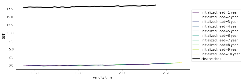
We have a huge bias because the initialized data is already converted to an anomaly, but uninitialized and observations is not. We also have a trend in all of our products, so we could also detrend them as well.
Detrend
We can leverage xarray’s .map() function to apply/map a function to all variables in our datasets. We use climpred.stats.rm_poly() to remove the trend.
from climpred.stats import rm_poly

hindcast_detrended = hindcast.map(rm_poly, deg=2, dim="init_or_time")
hindcast_detrended.plot()
<AxesSubplot:xlabel='validity time', ylabel='SST'>
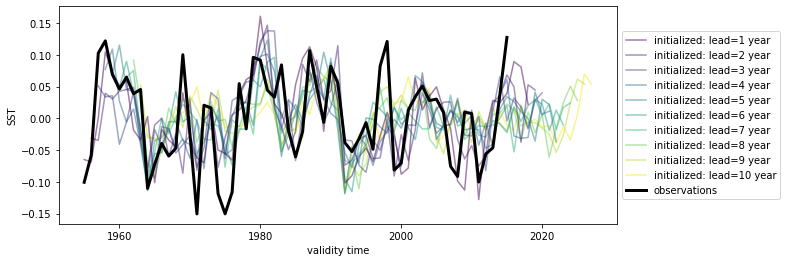
And it looks like everything got detrended by a quadratic fit! That wasn’t too hard.
Verify
Now that we’ve done our pre-processing, let’s quickly compute some metrics. Check the metrics for all the keywords you can use. The API is currently pretty simple for the HindcastEnsemble. You can essentially compute standard skill metrics and reference forecasts, here persistence.
hindcast_detrended.verify(
    metric="mse",
    comparison="e2o",
    dim="init",
    alignment="same_verif",
    reference="persistence",
)
<xarray.Dataset>
Dimensions:  (skill: 2, lead: 10)
Coordinates:
  * lead     (lead) int32 1 2 3 4 5 6 7 8 9 10
  * skill    (skill) <U11 'initialized' 'persistence'
Data variables:
    SST      (skill, lead) float64 0.003274 0.004149 ... 0.01109 0.008786
Attributes:
    prediction_skill_software:     climpred https://climpred.readthedocs.io/
    skill_calculated_by_function:  HindcastEnsemble.verify()
    number_of_initializations:     64
    alignment:                     same_verif
    metric:                        mse
    comparison:                    e2o
    dim:                           init
reference: ['persistence']- skill: 2
- lead: 10
- lead(lead)int321 2 3 4 5 6 7 8 9 10
- long_name :
- Lead
- units :
- years
- standard_name :
- forecast_period
- description :
- Forecast period is the time interval between the forecast reference time and the validity time. A period is an interval of time, or the time-period of an oscillation.
array([ 1, 2, 3, 4, 5, 6, 7, 8, 9, 10], dtype=int32)
- skill(skill)<U11'initialized' 'persistence'
- description :
- new dimension prediction skill of initialized and reference forecasts created by .verify() or .bootstrap()
- documentation :
- https://climpred.readthedocs.io/en/v2.1.7.dev40+ga522c2d.d20211213/reference_forecast.html
- initialized :
- initialized forecast skill
- persistence :
- persistence forecast skill
array(['initialized', 'persistence'], dtype='<U11')
- SST(skill, lead)float640.003274 0.004149 ... 0.008786
array([[0.00327367, 0.00414915, 0.00470421, 0.00396995, 0.00441036,
        0.00417693, 0.0042671 , 0.00424253, 0.00530586, 0.00549388],
       [0.0064499 , 0.01133794, 0.00940036, 0.00953341, 0.01158821,
        0.01120976, 0.00952641, 0.0100052 , 0.01108853, 0.00878648]])
- prediction_skill_software :
- climpred https://climpred.readthedocs.io/
- skill_calculated_by_function :
- HindcastEnsemble.verify()
- number_of_initializations :
- 64
- alignment :
- same_verif
- metric :
- mse
- comparison :
- e2o
- dim :
- init
- reference :
- ['persistence']
Here we leverage xarray’s plotting method to compute Mean Absolute Error and the Anomaly Correlation Coefficient against the ERSST observations, as well as the equivalent metrics computed for persistence forecasts for each of those metrics.
metrics = ["mae", "acc"]
for metric in metrics:
    hindcast_detrended.verify(
        metric=metric,
        comparison="e2o",
        dim="init",
        alignment="same_verif",
        reference="persistence",
    ).assign_coords(metric=metric.upper()).SST.plot(hue="skill")
    plt.suptitle("CESM Decadal Prediction Large Ensemble Global SSTs", fontsize=16)
    plt.show()
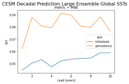
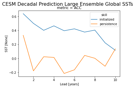
PerfectModelEnsemble
We’ll now play around a bit with the PerfectModelEnsemble object, using sample data from the MPI-ESM perfect model configuration.
initialized = load_dataset("MPI-PM-DP-1D")  # initialized ensemble from MPI
control = load_dataset("MPI-control-1D")  # base control run that initialized it

initialized["lead"].attrs["units"] = "years"
pm = climpred.PerfectModelEnsemble(initialized).add_control(control)
pm
/Users/aaron.spring/Coding/climpred/climpred/utils.py:191: UserWarning: Assuming annual resolution starting Jan 1st due to numeric inits. Please change ``init`` to a datetime if it is another resolution. We recommend using xr.CFTimeIndex as ``init``, see https://climpred.readthedocs.io/en/stable/setting-up-data.html.
  warnings.warn(
climpred.PerfectModelEnsemble
<Initialized Ensemble>
Dimensions:     (period: 5, lead: 20, area: 3, init: 12, member: 10)
Coordinates:
  * lead        (lead) int64 1 2 3 4 5 6 7 8 9 10 11 12 13 14 15 16 17 18 19 20
  * period      (period) object 'DJF' 'JJA' 'MAM' 'SON' 'ym'
  * area        (area) object 'global' 'North_Atlantic' 'North_Atlantic_SPG'
  * init        (init) object 3014-01-01 00:00:00 ... 3257-01-01 00:00:00
  * member      (member) int64 0 1 2 3 4 5 6 7 8 9
    valid_time  (lead, init) object 3015-01-01 00:00:00 ... 3277-01-01 00:00:00
Data variables:
    tos         (period, lead, area, init, member) float32 17.38 17.58 ... 8.955
    sos         (period, lead, area, init, member) float32 34.38 34.37 ... 34.59
AMO (period, lead, area, init, member) float32 0.1675 ... 0.06075- period: 5
- lead: 20
- area: 3
- init: 12
- member: 10
- lead(lead)int641 2 3 4 5 6 7 ... 15 16 17 18 19 20
- units :
- years
- standard_name :
- forecast_period
- long_name :
- Lead
- description :
- Forecast period is the time interval between the forecast reference time and the validity time. A period is an interval of time, or the time-period of an oscillation.
array([ 1, 2, 3, 4, 5, 6, 7, 8, 9, 10, 11, 12, 13, 14, 15, 16, 17, 18, 19, 20]) - period(period)object'DJF' 'JJA' 'MAM' 'SON' 'ym'
array(['DJF', 'JJA', 'MAM', 'SON', 'ym'], dtype=object)
- area(area)object'global' ... 'North_Atlantic_SPG'
array(['global', 'North_Atlantic', 'North_Atlantic_SPG'], dtype=object)
- init(init)object3014-01-01 00:00:00 ... 3257-01-...
- standard_name :
- forecast_reference_time
- long_name :
- Initialization
- description :
- The forecast reference time in NWP is the "data time", the time of the analysis from which the forecast was made. It is not the time for which the forecast is valid; the standard name of time should be used for that time.
array([cftime.DatetimeProlepticGregorian(3014, 1, 1, 0, 0, 0, 0, has_year_zero=True), cftime.DatetimeProlepticGregorian(3023, 1, 1, 0, 0, 0, 0, has_year_zero=True), cftime.DatetimeProlepticGregorian(3045, 1, 1, 0, 0, 0, 0, has_year_zero=True), cftime.DatetimeProlepticGregorian(3061, 1, 1, 0, 0, 0, 0, has_year_zero=True), cftime.DatetimeProlepticGregorian(3124, 1, 1, 0, 0, 0, 0, has_year_zero=True), cftime.DatetimeProlepticGregorian(3139, 1, 1, 0, 0, 0, 0, has_year_zero=True), cftime.DatetimeProlepticGregorian(3144, 1, 1, 0, 0, 0, 0, has_year_zero=True), cftime.DatetimeProlepticGregorian(3175, 1, 1, 0, 0, 0, 0, has_year_zero=True), cftime.DatetimeProlepticGregorian(3178, 1, 1, 0, 0, 0, 0, has_year_zero=True), cftime.DatetimeProlepticGregorian(3228, 1, 1, 0, 0, 0, 0, has_year_zero=True), cftime.DatetimeProlepticGregorian(3237, 1, 1, 0, 0, 0, 0, has_year_zero=True), cftime.DatetimeProlepticGregorian(3257, 1, 1, 0, 0, 0, 0, has_year_zero=True)], dtype=object) - member(member)int640 1 2 3 4 5 6 7 8 9
- standard_name :
- realization
- long_name :
- Member
- description :
- Realization is used to label a dimension that can be thought of as a statistical sample, e.g., labelling members of a model ensemble.
array([0, 1, 2, 3, 4, 5, 6, 7, 8, 9])
- valid_time(lead, init)object3015-01-01 00:00:00 ... 3277-01-...
- long_name :
- validity time
- standard_name :
- time
- description :
- time for which the forecast is valid
- calculate :
- init + lead
- amip :
- time
array([[cftime.DatetimeProlepticGregorian(3015, 1, 1, 0, 0, 0, 0, has_year_zero=True),
        cftime.DatetimeProlepticGregorian(3024, 1, 1, 0, 0, 0, 0, has_year_zero=True),
        cftime.DatetimeProlepticGregorian(3046, 1, 1, 0, 0, 0, 0, has_year_zero=True),
        cftime.DatetimeProlepticGregorian(3062, 1, 1, 0, 0, 0, 0, has_year_zero=True),
        cftime.DatetimeProlepticGregorian(3125, 1, 1, 0, 0, 0, 0, has_year_zero=True),
        cftime.DatetimeProlepticGregorian(3140, 1, 1, 0, 0, 0, 0, has_year_zero=True),
        cftime.DatetimeProlepticGregorian(3145, 1, 1, 0, 0, 0, 0, has_year_zero=True),
        cftime.DatetimeProlepticGregorian(3176, 1, 1, 0, 0, 0, 0, has_year_zero=True),
        cftime.DatetimeProlepticGregorian(3179, 1, 1, 0, 0, 0, 0, has_year_zero=True),
        cftime.DatetimeProlepticGregorian(3229, 1, 1, 0, 0, 0, 0, has_year_zero=True),
        cftime.DatetimeProlepticGregorian(3238, 1, 1, 0, 0, 0, 0, has_year_zero=True),
        cftime.DatetimeProlepticGregorian(3258, 1, 1, 0, 0, 0, 0, has_year_zero=True)],
       [cftime.DatetimeProlepticGregorian(3016, 1, 1, 0, 0, 0, 0, has_year_zero=True),
        cftime.DatetimeProlepticGregorian(3025, 1, 1, 0, 0, 0, 0, has_year_zero=True),
        cftime.DatetimeProlepticGregorian(3047, 1, 1, 0, 0, 0, 0, has_year_zero=True),
        cftime.DatetimeProlepticGregorian(3063, 1, 1, 0, 0, 0, 0, has_year_zero=True),
        cftime.DatetimeProlepticGregorian(3126, 1, 1, 0, 0, 0, 0, has_year_zero=True),
        cftime.DatetimeProlepticGregorian(3141, 1, 1, 0, 0, 0, 0, has_year_zero=True),
        cftime.DatetimeProlepticGregorian(3146, 1, 1, 0, 0, 0, 0, has_year_zero=True),
        cftime.DatetimeProlepticGregorian(3177, 1, 1, 0, 0, 0, 0, has_year_zero=True),
...
        cftime.DatetimeProlepticGregorian(3158, 1, 1, 0, 0, 0, 0, has_year_zero=True),
        cftime.DatetimeProlepticGregorian(3163, 1, 1, 0, 0, 0, 0, has_year_zero=True),
        cftime.DatetimeProlepticGregorian(3194, 1, 1, 0, 0, 0, 0, has_year_zero=True),
        cftime.DatetimeProlepticGregorian(3197, 1, 1, 0, 0, 0, 0, has_year_zero=True),
        cftime.DatetimeProlepticGregorian(3247, 1, 1, 0, 0, 0, 0, has_year_zero=True),
        cftime.DatetimeProlepticGregorian(3256, 1, 1, 0, 0, 0, 0, has_year_zero=True),
        cftime.DatetimeProlepticGregorian(3276, 1, 1, 0, 0, 0, 0, has_year_zero=True)],
       [cftime.DatetimeProlepticGregorian(3034, 1, 1, 0, 0, 0, 0, has_year_zero=True),
        cftime.DatetimeProlepticGregorian(3043, 1, 1, 0, 0, 0, 0, has_year_zero=True),
        cftime.DatetimeProlepticGregorian(3065, 1, 1, 0, 0, 0, 0, has_year_zero=True),
        cftime.DatetimeProlepticGregorian(3081, 1, 1, 0, 0, 0, 0, has_year_zero=True),
        cftime.DatetimeProlepticGregorian(3144, 1, 1, 0, 0, 0, 0, has_year_zero=True),
        cftime.DatetimeProlepticGregorian(3159, 1, 1, 0, 0, 0, 0, has_year_zero=True),
        cftime.DatetimeProlepticGregorian(3164, 1, 1, 0, 0, 0, 0, has_year_zero=True),
        cftime.DatetimeProlepticGregorian(3195, 1, 1, 0, 0, 0, 0, has_year_zero=True),
        cftime.DatetimeProlepticGregorian(3198, 1, 1, 0, 0, 0, 0, has_year_zero=True),
        cftime.DatetimeProlepticGregorian(3248, 1, 1, 0, 0, 0, 0, has_year_zero=True),
        cftime.DatetimeProlepticGregorian(3257, 1, 1, 0, 0, 0, 0, has_year_zero=True),
        cftime.DatetimeProlepticGregorian(3277, 1, 1, 0, 0, 0, 0, has_year_zero=True)]],
      dtype=object)
- tos(period, lead, area, init, member)float3217.38 17.58 17.46 ... 8.781 8.955
array([[[[[17.384073, ..., 17.389244], ..., [17.49527 , ..., 17.647034]], ..., [[ 7.004498, ..., 6.904807], ..., [ 7.15443 , ..., 6.934058]]], ..., [[[17.349993, ..., 17.345932], ..., [17.387072, ..., 17.506124]], ..., [[ 7.208045, ..., 6.726819], ..., [ 6.953272, ..., 7.062301]]]], ..., [[[[17.304762, ..., 17.2879 ], ..., [17.282705, ..., 17.358082]], ..., [[ 8.295001, ..., 8.414991], ..., [ 8.457472, ..., 8.715961]]], ..., [[[17.28034 , ..., 17.199175], ..., [17.197533, ..., 17.290545]], ..., [[ 9.117534, ..., 8.16558 ], ..., [ 8.585161, ..., 8.954581]]]]], dtype=float32) - sos(period, lead, area, init, member)float3234.38 34.37 34.39 ... 34.61 34.59
array([[[[[34.381344, ..., 34.395466], ..., [34.379017, ..., 34.375397]], ..., [[34.621056, ..., 34.490482], ..., [34.73688 , ..., 34.667927]]], ..., [[[34.367462, ..., 34.3745 ], ..., [34.382206, ..., 34.3752 ]], ..., [[34.71535 , ..., 34.644875], ..., [34.60751 , ..., 34.749866]]]], ..., [[[[34.371273, ..., 34.377483], ..., [34.367928, ..., 34.367786]], ..., [[34.54275 , ..., 34.46146 ], ..., [34.542786, ..., 34.631397]]], ..., [[[34.360554, ..., 34.368996], ..., [34.37161 , ..., 34.35645 ]], ..., [[34.622524, ..., 34.52258 ], ..., [34.527443, ..., 34.587795]]]]], dtype=float32) - AMO(period, lead, area, init, member)float320.1675 0.02531 ... -0.01757 0.06075
array([[[[[ 0.167495, ...,  0.047088],
          ...,
          [-0.232761, ..., -0.273002]],

         ...,

         [[ 0.167495, ...,  0.047088],
          ...,
          [-0.232761, ..., -0.273002]]],


        ...,


        [[[ 0.273698, ..., -0.124981],
          ...,
          [-0.002182, ..., -0.01367 ]],

         ...,

         [[ 0.273698, ..., -0.124981],
          ...,
          [-0.002182, ..., -0.01367 ]]]],


       ...,


       [[[[ 0.072317, ...,  0.139705],
          ...,
          [-0.208696, ..., -0.327045]],

         ...,

         [[ 0.072317, ...,  0.139705],
          ...,
          [-0.208696, ..., -0.327045]]],


        ...,


        [[[ 0.325681, ..., -0.209799],
          ...,
          [-0.01501 , ...,  0.060747]],

         ...,

         [[ 0.325681, ..., -0.209799],
          ...,
          [-0.01501 , ...,  0.060747]]]]], dtype=float32)
<Control Simulation>
Dimensions:  (period: 5, time: 300, area: 3)
Coordinates:
  * time     (time) object 3000-01-01 00:00:00 ... 3299-01-01 00:00:00
  * period   (period) object 'DJF' 'JJA' 'MAM' 'SON' 'ym'
  * area     (area) object 'global' 'North_Atlantic' 'North_Atlantic_SPG'
Data variables:
    tos      (period, time, area) float32 17.38 8.76 7.321 ... 17.23 10.84 8.346
    sos      (period, time, area) float32 34.37 33.5 34.72 ... 34.35 33.38 34.45
AMO (period, time, area) float32 0.17 0.17 0.17 ... 0.07905 0.07905- period: 5
- time: 300
- area: 3
- time(time)object3000-01-01 00:00:00 ... 3299-01-...
- long_name :
- time
- standard_name :
- time
array([cftime.DatetimeProlepticGregorian(3000, 1, 1, 0, 0, 0, 0, has_year_zero=True), cftime.DatetimeProlepticGregorian(3001, 1, 1, 0, 0, 0, 0, has_year_zero=True), cftime.DatetimeProlepticGregorian(3002, 1, 1, 0, 0, 0, 0, has_year_zero=True), ..., cftime.DatetimeProlepticGregorian(3297, 1, 1, 0, 0, 0, 0, has_year_zero=True), cftime.DatetimeProlepticGregorian(3298, 1, 1, 0, 0, 0, 0, has_year_zero=True), cftime.DatetimeProlepticGregorian(3299, 1, 1, 0, 0, 0, 0, has_year_zero=True)], dtype=object) - period(period)object'DJF' 'JJA' 'MAM' 'SON' 'ym'
array(['DJF', 'JJA', 'MAM', 'SON', 'ym'], dtype=object)
- area(area)object'global' ... 'North_Atlantic_SPG'
array(['global', 'North_Atlantic', 'North_Atlantic_SPG'], dtype=object)
- tos(period, time, area)float3217.38 8.76 7.321 ... 10.84 8.346
array([[[17.382196, 8.759807, 7.320567], [17.344793, 8.402126, 7.033539], ..., [17.406504, 8.515713, 6.448978], [17.368383, 8.417525, 6.937928]], [[17.159786, 13.499312, 10.919159], [17.00704 , 13.742612, 11.459312], ..., [17.085367, 13.076672, 9.879821], [17.125288, 13.465583, 10.465502]], ..., [[16.988144, 13.185364, 10.20008 ], [16.88766 , 13.153466, 9.775887], ..., [16.989845, 12.697525, 9.045184], [16.961275, 13.096062, 9.693774]], [[17.301888, 10.906495, 8.973052], [17.148916, 10.958404, 8.937663], ..., [17.221823, 10.586926, 7.862315], [17.232193, 10.836343, 8.346231]]], dtype=float32) - sos(period, time, area)float3234.37 33.5 34.72 ... 33.38 34.45
array([[[34.371998, 33.502525, 34.719456], [34.355347, 33.519848, 34.671505], ..., [34.365993, 33.568325, 34.630814], [34.355545, 33.500748, 34.479523]], [[34.33216 , 33.232624, 34.601894], [34.330135, 33.188156, 34.487717], ..., [34.32915 , 33.16359 , 34.32454 ], [34.330036, 33.18352 , 34.319214]], ..., [[34.33014 , 33.288124, 34.564205], [34.326954, 33.26364 , 34.474926], ..., [34.320232, 33.2581 , 34.364594], [34.32564 , 33.225998, 34.278736]], [[34.357925, 33.449768, 34.69097 ], [34.355095, 33.3701 , 34.60008 ], ..., [34.35066 , 33.391457, 34.48565 ], [34.353535, 33.38208 , 34.451256]]], dtype=float32) - AMO(period, time, area)float320.17 0.17 0.17 ... 0.07905 0.07905
array([[[ 0.169961,  0.169961,  0.169961],
        [-0.103922, -0.103922, -0.103922],
        ...,
        [ 0.117817,  0.117817,  0.117817],
        [-0.032913, -0.032913, -0.032913]],

       [[ 0.234705,  0.234705,  0.234705],
        [ 0.267132,  0.267132,  0.267132],
        ...,
        [-0.13114 , -0.13114 , -0.13114 ],
        [ 0.036084,  0.036084,  0.036084]],

       ...,

       [[ 0.142128,  0.142128,  0.142128],
        [ 0.087876,  0.087876,  0.087876],
        ...,
        [-0.086413, -0.086413, -0.086413],
        [ 0.151093,  0.151093,  0.151093]],

       [[ 0.167775,  0.167775,  0.167775],
        [ 0.161447,  0.161447,  0.161447],
        ...,
        [-0.02503 , -0.02503 , -0.02503 ],
        [ 0.079047,  0.079047,  0.079047]]], dtype=float32)
Our objects are carrying sea surface temperature (tos), sea surface salinity (sos), and the Atlantic Multidecadal Oscillation index (AMO). Say we just want to look at skill metrics for temperature and salinity over the North Atlantic in JJA. We can just call a few easy xarray commands to filter down our object.
pm = pm[["tos", "sos"]].sel(area="North_Atlantic", period="JJA", drop=True)
Now we can easily compute for a host of metrics. Here I just show a number of deterministic skill metrics comparing all individual members to the initialized ensemble mean. See comparisons for more information on the comparison keyword.
METRICS = ["mse", "rmse", "mae", "acc", "nmse", "nrmse", "nmae", "msss"]

result = []
for metric in METRICS:
    result.append(pm.verify(metric=metric, comparison="m2e", dim=["init", "member"]))

result = xr.concat(result, "metric")
result["metric"] = METRICS

# Leverage the `xarray` plotting wrapper to plot all results at once.
result.to_array().plot(
    col="metric", hue="variable", col_wrap=4, sharey=False, sharex=True
)
<xarray.plot.facetgrid.FacetGrid at 0x14febcb20>
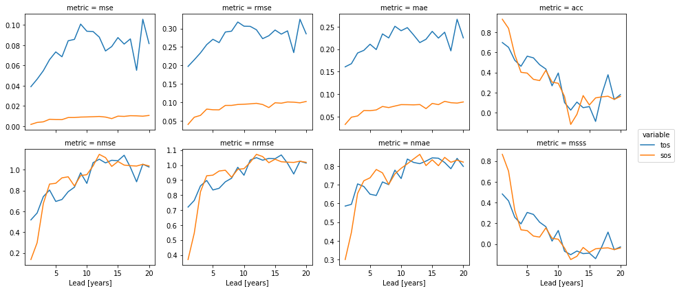
It is useful to compare the initialized ensemble to an uninitialized run. See terminology for a description on uninitialized simulations. This gives us information about how initialization leads to enhanced predictability over knowledge of external forcing, whereas a comparison to persistence just tells us how well a dynamical forecast simulation does in comparison to a naive method. We can use the PerfectModelEnsemble.generate_uninitialized() to resample the control run and create a pseudo-ensemble that approximates what an uninitialized ensemble would look like.
pm = pm.generate_uninitialized()
pm
climpred.PerfectModelEnsemble
<Initialized Ensemble>
Dimensions:     (lead: 20, init: 12, member: 10)
Coordinates:
  * lead        (lead) int64 1 2 3 4 5 6 7 8 9 10 11 12 13 14 15 16 17 18 19 20
  * init        (init) object 3014-01-01 00:00:00 ... 3257-01-01 00:00:00
  * member      (member) int64 0 1 2 3 4 5 6 7 8 9
    valid_time  (lead, init) object 3015-01-01 00:00:00 ... 3277-01-01 00:00:00
Data variables:
    tos         (lead, init, member) float32 13.46 13.64 13.72 ... 13.55 13.57
sos (lead, init, member) float32 33.18 33.15 33.05 ... 33.18 33.26- lead: 20
- init: 12
- member: 10
- lead(lead)int641 2 3 4 5 6 7 ... 15 16 17 18 19 20
- units :
- years
- standard_name :
- forecast_period
- long_name :
- Lead
- description :
- Forecast period is the time interval between the forecast reference time and the validity time. A period is an interval of time, or the time-period of an oscillation.
array([ 1, 2, 3, 4, 5, 6, 7, 8, 9, 10, 11, 12, 13, 14, 15, 16, 17, 18, 19, 20]) - init(init)object3014-01-01 00:00:00 ... 3257-01-...
- standard_name :
- forecast_reference_time
- long_name :
- Initialization
- description :
- The forecast reference time in NWP is the "data time", the time of the analysis from which the forecast was made. It is not the time for which the forecast is valid; the standard name of time should be used for that time.
array([cftime.DatetimeProlepticGregorian(3014, 1, 1, 0, 0, 0, 0, has_year_zero=True), cftime.DatetimeProlepticGregorian(3023, 1, 1, 0, 0, 0, 0, has_year_zero=True), cftime.DatetimeProlepticGregorian(3045, 1, 1, 0, 0, 0, 0, has_year_zero=True), cftime.DatetimeProlepticGregorian(3061, 1, 1, 0, 0, 0, 0, has_year_zero=True), cftime.DatetimeProlepticGregorian(3124, 1, 1, 0, 0, 0, 0, has_year_zero=True), cftime.DatetimeProlepticGregorian(3139, 1, 1, 0, 0, 0, 0, has_year_zero=True), cftime.DatetimeProlepticGregorian(3144, 1, 1, 0, 0, 0, 0, has_year_zero=True), cftime.DatetimeProlepticGregorian(3175, 1, 1, 0, 0, 0, 0, has_year_zero=True), cftime.DatetimeProlepticGregorian(3178, 1, 1, 0, 0, 0, 0, has_year_zero=True), cftime.DatetimeProlepticGregorian(3228, 1, 1, 0, 0, 0, 0, has_year_zero=True), cftime.DatetimeProlepticGregorian(3237, 1, 1, 0, 0, 0, 0, has_year_zero=True), cftime.DatetimeProlepticGregorian(3257, 1, 1, 0, 0, 0, 0, has_year_zero=True)], dtype=object) - member(member)int640 1 2 3 4 5 6 7 8 9
- standard_name :
- realization
- long_name :
- Member
- description :
- Realization is used to label a dimension that can be thought of as a statistical sample, e.g., labelling members of a model ensemble.
array([0, 1, 2, 3, 4, 5, 6, 7, 8, 9])
- valid_time(lead, init)object3015-01-01 00:00:00 ... 3277-01-...
- long_name :
- validity time
- standard_name :
- time
- description :
- time for which the forecast is valid
- calculate :
- init + lead
- amip :
- time
array([[cftime.DatetimeProlepticGregorian(3015, 1, 1, 0, 0, 0, 0, has_year_zero=True),
        cftime.DatetimeProlepticGregorian(3024, 1, 1, 0, 0, 0, 0, has_year_zero=True),
        cftime.DatetimeProlepticGregorian(3046, 1, 1, 0, 0, 0, 0, has_year_zero=True),
        cftime.DatetimeProlepticGregorian(3062, 1, 1, 0, 0, 0, 0, has_year_zero=True),
        cftime.DatetimeProlepticGregorian(3125, 1, 1, 0, 0, 0, 0, has_year_zero=True),
        cftime.DatetimeProlepticGregorian(3140, 1, 1, 0, 0, 0, 0, has_year_zero=True),
        cftime.DatetimeProlepticGregorian(3145, 1, 1, 0, 0, 0, 0, has_year_zero=True),
        cftime.DatetimeProlepticGregorian(3176, 1, 1, 0, 0, 0, 0, has_year_zero=True),
        cftime.DatetimeProlepticGregorian(3179, 1, 1, 0, 0, 0, 0, has_year_zero=True),
        cftime.DatetimeProlepticGregorian(3229, 1, 1, 0, 0, 0, 0, has_year_zero=True),
        cftime.DatetimeProlepticGregorian(3238, 1, 1, 0, 0, 0, 0, has_year_zero=True),
        cftime.DatetimeProlepticGregorian(3258, 1, 1, 0, 0, 0, 0, has_year_zero=True)],
       [cftime.DatetimeProlepticGregorian(3016, 1, 1, 0, 0, 0, 0, has_year_zero=True),
        cftime.DatetimeProlepticGregorian(3025, 1, 1, 0, 0, 0, 0, has_year_zero=True),
        cftime.DatetimeProlepticGregorian(3047, 1, 1, 0, 0, 0, 0, has_year_zero=True),
        cftime.DatetimeProlepticGregorian(3063, 1, 1, 0, 0, 0, 0, has_year_zero=True),
        cftime.DatetimeProlepticGregorian(3126, 1, 1, 0, 0, 0, 0, has_year_zero=True),
        cftime.DatetimeProlepticGregorian(3141, 1, 1, 0, 0, 0, 0, has_year_zero=True),
        cftime.DatetimeProlepticGregorian(3146, 1, 1, 0, 0, 0, 0, has_year_zero=True),
        cftime.DatetimeProlepticGregorian(3177, 1, 1, 0, 0, 0, 0, has_year_zero=True),
...
        cftime.DatetimeProlepticGregorian(3158, 1, 1, 0, 0, 0, 0, has_year_zero=True),
        cftime.DatetimeProlepticGregorian(3163, 1, 1, 0, 0, 0, 0, has_year_zero=True),
        cftime.DatetimeProlepticGregorian(3194, 1, 1, 0, 0, 0, 0, has_year_zero=True),
        cftime.DatetimeProlepticGregorian(3197, 1, 1, 0, 0, 0, 0, has_year_zero=True),
        cftime.DatetimeProlepticGregorian(3247, 1, 1, 0, 0, 0, 0, has_year_zero=True),
        cftime.DatetimeProlepticGregorian(3256, 1, 1, 0, 0, 0, 0, has_year_zero=True),
        cftime.DatetimeProlepticGregorian(3276, 1, 1, 0, 0, 0, 0, has_year_zero=True)],
       [cftime.DatetimeProlepticGregorian(3034, 1, 1, 0, 0, 0, 0, has_year_zero=True),
        cftime.DatetimeProlepticGregorian(3043, 1, 1, 0, 0, 0, 0, has_year_zero=True),
        cftime.DatetimeProlepticGregorian(3065, 1, 1, 0, 0, 0, 0, has_year_zero=True),
        cftime.DatetimeProlepticGregorian(3081, 1, 1, 0, 0, 0, 0, has_year_zero=True),
        cftime.DatetimeProlepticGregorian(3144, 1, 1, 0, 0, 0, 0, has_year_zero=True),
        cftime.DatetimeProlepticGregorian(3159, 1, 1, 0, 0, 0, 0, has_year_zero=True),
        cftime.DatetimeProlepticGregorian(3164, 1, 1, 0, 0, 0, 0, has_year_zero=True),
        cftime.DatetimeProlepticGregorian(3195, 1, 1, 0, 0, 0, 0, has_year_zero=True),
        cftime.DatetimeProlepticGregorian(3198, 1, 1, 0, 0, 0, 0, has_year_zero=True),
        cftime.DatetimeProlepticGregorian(3248, 1, 1, 0, 0, 0, 0, has_year_zero=True),
        cftime.DatetimeProlepticGregorian(3257, 1, 1, 0, 0, 0, 0, has_year_zero=True),
        cftime.DatetimeProlepticGregorian(3277, 1, 1, 0, 0, 0, 0, has_year_zero=True)]],
      dtype=object)
- tos(lead, init, member)float3213.46 13.64 13.72 ... 13.55 13.57
array([[[13.464135, 13.641711, ..., 13.588738, 13.266194], [13.445477, 13.571556, ..., 13.525509, 13.063034], ..., [12.837116, 13.368766, ..., 12.992356, 12.98161 ], [12.917976, 13.191601, ..., 12.989105, 12.764714]], [[13.744945, 13.574756, ..., 13.699843, 13.458035], [13.599129, 13.605476, ..., 13.617603, 13.762051], ..., [12.549422, 13.148598, ..., 12.93991 , 12.665627], [13.0729 , 13.025772, ..., 13.134182, 13.14777 ]], ..., [[13.504623, 13.638802, ..., 13.734439, 13.001564], [13.149283, 13.082256, ..., 13.71314 , 13.515602], ..., [13.211761, 13.369294, ..., 12.697314, 13.112003], [13.114143, 13.344111, ..., 12.86262 , 13.52319 ]], [[13.923348, 13.569972, ..., 13.548902, 13.060498], [13.192071, 13.177944, ..., 13.212311, 13.26723 ], ..., [13.196457, 13.203984, ..., 12.743962, 12.803421], [13.555382, 13.436454, ..., 13.547691, 13.568891]]], dtype=float32) - sos(lead, init, member)float3233.18 33.15 33.05 ... 33.18 33.26
array([[[33.183903, 33.146976, ..., 33.14601 , 33.09485 ],
        [33.169205, 33.154438, ..., 33.137466, 33.168583],
        ...,
        [32.995815, 32.983433, ..., 33.031227, 32.99914 ],
        [33.05064 , 33.114414, ..., 32.998016, 33.093204]],

       [[33.199635, 33.082794, ..., 33.234913, 33.11563 ],
        [33.144375, 33.187267, ..., 33.110977, 33.18133 ],
        ...,
        [33.081043, 33.05753 , ..., 33.098064, 32.96622 ],
        [33.104546, 33.033073, ..., 32.976826, 33.069054]],

       ...,

       [[33.174488, 33.30829 , ..., 33.105885, 32.935608],
        [33.13984 , 33.22768 , ..., 33.123425, 33.11398 ],
        ...,
        [33.17692 , 33.119602, ..., 32.99104 , 33.063793],
        [33.196835, 33.186802, ..., 33.227722, 33.400288]],

       [[33.136868, 33.354904, ..., 33.147465, 33.092255],
        [33.178905, 33.15257 , ..., 33.097546, 33.223183],
        ...,
        [32.995438, 33.067974, ..., 32.925762, 32.951527],
        [33.19941 , 33.20508 , ..., 33.18124 , 33.25843 ]]], dtype=float32)
<Control Simulation>
Dimensions:  (time: 300)
Coordinates:
  * time     (time) object 3000-01-01 00:00:00 ... 3299-01-01 00:00:00
Data variables:
    tos      (time) float32 13.5 13.74 13.78 13.86 ... 13.12 12.92 13.08 13.47
sos (time) float32 33.23 33.19 33.2 33.21 ... 33.15 33.22 33.16 33.18- time: 300
- time(time)object3000-01-01 00:00:00 ... 3299-01-...
- long_name :
- time
- standard_name :
- time
array([cftime.DatetimeProlepticGregorian(3000, 1, 1, 0, 0, 0, 0, has_year_zero=True),
       cftime.DatetimeProlepticGregorian(3001, 1, 1, 0, 0, 0, 0, has_year_zero=True),
       cftime.DatetimeProlepticGregorian(3002, 1, 1, 0, 0, 0, 0, has_year_zero=True),
       ...,
       cftime.DatetimeProlepticGregorian(3297, 1, 1, 0, 0, 0, 0, has_year_zero=True),
       cftime.DatetimeProlepticGregorian(3298, 1, 1, 0, 0, 0, 0, has_year_zero=True),
       cftime.DatetimeProlepticGregorian(3299, 1, 1, 0, 0, 0, 0, has_year_zero=True)],
      dtype=object)
- tos(time)float3213.5 13.74 13.78 ... 13.08 13.47
array([13.499312, 13.742612, 13.783769, ..., 12.917691, 13.076672, 13.465583], dtype=float32) - sos(time)float3233.23 33.19 33.2 ... 33.16 33.18
array([33.232624, 33.188156, 33.201694, ..., 33.221058, 33.16359 , 33.18352 ],
      dtype=float32)
<Uninitialized>
Dimensions:     (lead: 20, init: 12, member: 10)
Coordinates:
    valid_time  (lead, init) object 3015-01-01 00:00:00 ... 3277-01-01 00:00:00
  * lead        (lead) int64 1 2 3 4 5 6 7 8 9 10 11 12 13 14 15 16 17 18 19 20
  * init        (init) object 3014-01-01 00:00:00 ... 3257-01-01 00:00:00
  * member      (member) int64 0 1 2 3 4 5 6 7 8 9
Data variables:
    tos         (lead, init, member) float32 13.01 12.84 12.84 ... 13.44 13.57
sos (lead, init, member) float32 33.08 33.08 33.0 ... 33.16 33.32- lead: 20
- init: 12
- member: 10
- valid_time(lead, init)object3015-01-01 00:00:00 ... 3277-01-...
- long_name :
- validity time
- standard_name :
- time
- description :
- time for which the forecast is valid
- calculate :
- init + lead
- amip :
- time
array([[cftime.DatetimeProlepticGregorian(3015, 1, 1, 0, 0, 0, 0, has_year_zero=True), cftime.DatetimeProlepticGregorian(3024, 1, 1, 0, 0, 0, 0, has_year_zero=True), cftime.DatetimeProlepticGregorian(3046, 1, 1, 0, 0, 0, 0, has_year_zero=True), cftime.DatetimeProlepticGregorian(3062, 1, 1, 0, 0, 0, 0, has_year_zero=True), cftime.DatetimeProlepticGregorian(3125, 1, 1, 0, 0, 0, 0, has_year_zero=True), cftime.DatetimeProlepticGregorian(3140, 1, 1, 0, 0, 0, 0, has_year_zero=True), cftime.DatetimeProlepticGregorian(3145, 1, 1, 0, 0, 0, 0, has_year_zero=True), cftime.DatetimeProlepticGregorian(3176, 1, 1, 0, 0, 0, 0, has_year_zero=True), cftime.DatetimeProlepticGregorian(3179, 1, 1, 0, 0, 0, 0, has_year_zero=True), cftime.DatetimeProlepticGregorian(3229, 1, 1, 0, 0, 0, 0, has_year_zero=True), cftime.DatetimeProlepticGregorian(3238, 1, 1, 0, 0, 0, 0, has_year_zero=True), cftime.DatetimeProlepticGregorian(3258, 1, 1, 0, 0, 0, 0, has_year_zero=True)], [cftime.DatetimeProlepticGregorian(3016, 1, 1, 0, 0, 0, 0, has_year_zero=True), cftime.DatetimeProlepticGregorian(3025, 1, 1, 0, 0, 0, 0, has_year_zero=True), cftime.DatetimeProlepticGregorian(3047, 1, 1, 0, 0, 0, 0, has_year_zero=True), cftime.DatetimeProlepticGregorian(3063, 1, 1, 0, 0, 0, 0, has_year_zero=True), cftime.DatetimeProlepticGregorian(3126, 1, 1, 0, 0, 0, 0, has_year_zero=True), cftime.DatetimeProlepticGregorian(3141, 1, 1, 0, 0, 0, 0, has_year_zero=True), cftime.DatetimeProlepticGregorian(3146, 1, 1, 0, 0, 0, 0, has_year_zero=True), cftime.DatetimeProlepticGregorian(3177, 1, 1, 0, 0, 0, 0, has_year_zero=True), ... cftime.DatetimeProlepticGregorian(3158, 1, 1, 0, 0, 0, 0, has_year_zero=True), cftime.DatetimeProlepticGregorian(3163, 1, 1, 0, 0, 0, 0, has_year_zero=True), cftime.DatetimeProlepticGregorian(3194, 1, 1, 0, 0, 0, 0, has_year_zero=True), cftime.DatetimeProlepticGregorian(3197, 1, 1, 0, 0, 0, 0, has_year_zero=True), cftime.DatetimeProlepticGregorian(3247, 1, 1, 0, 0, 0, 0, has_year_zero=True), cftime.DatetimeProlepticGregorian(3256, 1, 1, 0, 0, 0, 0, has_year_zero=True), cftime.DatetimeProlepticGregorian(3276, 1, 1, 0, 0, 0, 0, has_year_zero=True)], [cftime.DatetimeProlepticGregorian(3034, 1, 1, 0, 0, 0, 0, has_year_zero=True), cftime.DatetimeProlepticGregorian(3043, 1, 1, 0, 0, 0, 0, has_year_zero=True), cftime.DatetimeProlepticGregorian(3065, 1, 1, 0, 0, 0, 0, has_year_zero=True), cftime.DatetimeProlepticGregorian(3081, 1, 1, 0, 0, 0, 0, has_year_zero=True), cftime.DatetimeProlepticGregorian(3144, 1, 1, 0, 0, 0, 0, has_year_zero=True), cftime.DatetimeProlepticGregorian(3159, 1, 1, 0, 0, 0, 0, has_year_zero=True), cftime.DatetimeProlepticGregorian(3164, 1, 1, 0, 0, 0, 0, has_year_zero=True), cftime.DatetimeProlepticGregorian(3195, 1, 1, 0, 0, 0, 0, has_year_zero=True), cftime.DatetimeProlepticGregorian(3198, 1, 1, 0, 0, 0, 0, has_year_zero=True), cftime.DatetimeProlepticGregorian(3248, 1, 1, 0, 0, 0, 0, has_year_zero=True), cftime.DatetimeProlepticGregorian(3257, 1, 1, 0, 0, 0, 0, has_year_zero=True), cftime.DatetimeProlepticGregorian(3277, 1, 1, 0, 0, 0, 0, has_year_zero=True)]], dtype=object) - lead(lead)int641 2 3 4 5 6 7 ... 15 16 17 18 19 20
- units :
- years
- standard_name :
- forecast_period
- long_name :
- Lead
- description :
- Forecast period is the time interval between the forecast reference time and the validity time. A period is an interval of time, or the time-period of an oscillation.
array([ 1, 2, 3, 4, 5, 6, 7, 8, 9, 10, 11, 12, 13, 14, 15, 16, 17, 18, 19, 20]) - init(init)object3014-01-01 00:00:00 ... 3257-01-...
- standard_name :
- forecast_reference_time
- long_name :
- Initialization
- description :
- The forecast reference time in NWP is the "data time", the time of the analysis from which the forecast was made. It is not the time for which the forecast is valid; the standard name of time should be used for that time.
array([cftime.DatetimeProlepticGregorian(3014, 1, 1, 0, 0, 0, 0, has_year_zero=True), cftime.DatetimeProlepticGregorian(3023, 1, 1, 0, 0, 0, 0, has_year_zero=True), cftime.DatetimeProlepticGregorian(3045, 1, 1, 0, 0, 0, 0, has_year_zero=True), cftime.DatetimeProlepticGregorian(3061, 1, 1, 0, 0, 0, 0, has_year_zero=True), cftime.DatetimeProlepticGregorian(3124, 1, 1, 0, 0, 0, 0, has_year_zero=True), cftime.DatetimeProlepticGregorian(3139, 1, 1, 0, 0, 0, 0, has_year_zero=True), cftime.DatetimeProlepticGregorian(3144, 1, 1, 0, 0, 0, 0, has_year_zero=True), cftime.DatetimeProlepticGregorian(3175, 1, 1, 0, 0, 0, 0, has_year_zero=True), cftime.DatetimeProlepticGregorian(3178, 1, 1, 0, 0, 0, 0, has_year_zero=True), cftime.DatetimeProlepticGregorian(3228, 1, 1, 0, 0, 0, 0, has_year_zero=True), cftime.DatetimeProlepticGregorian(3237, 1, 1, 0, 0, 0, 0, has_year_zero=True), cftime.DatetimeProlepticGregorian(3257, 1, 1, 0, 0, 0, 0, has_year_zero=True)], dtype=object) - member(member)int640 1 2 3 4 5 6 7 8 9
array([0, 1, 2, 3, 4, 5, 6, 7, 8, 9])
- tos(lead, init, member)float3213.01 12.84 12.84 ... 13.44 13.57
array([[[13.009304 , 12.844365 , 12.837116 , ..., 13.011107 , 12.870223 , 13.160767 ], [13.067849 , 13.068427 , 13.627881 , ..., 13.137523 , 13.065289 , 13.663853 ], [13.113345 , 12.935954 , 13.188503 , ..., 13.349854 , 13.34776 , 13.729529 ], ..., [13.429088 , 13.483514 , 13.7393265, ..., 13.368962 , 13.105531 , 13.2029 ], [14.046454 , 13.454182 , 12.743481 , ..., 13.687771 , 13.646142 , 13.420696 ], [13.933627 , 13.972522 , 14.041756 , ..., 13.21655 , 13.226235 , 12.852818 ]], [[13.57552 , 12.935834 , 13.445477 , ..., 13.370051 , 13.359902 , 13.558215 ], [13.905151 , 13.504623 , 13.923348 , ..., 13.446274 , 13.426196 , 13.397359 ], [13.188503 , 13.011261 , 13.436942 , ..., 13.729529 , 13.242668 , 13.322024 ], ... [13.224067 , 12.829465 , 13.21901 , ..., 13.011261 , 13.436942 , 13.313319 ], [13.634433 , 13.7028475, 13.57552 , ..., 13.3854065, 13.456145 , 13.370051 ], [13.359902 , 13.558215 , 13.905151 , ..., 13.567241 , 14.031241 , 13.446274 ]], [[13.663853 , 13.211761 , 13.196457 , ..., 13.65322 , 13.455567 , 13.355483 ], [13.746189 , 13.501628 , 13.477757 , ..., 13.741005 , 13.592628 , 12.733609 ], [13.646504 , 13.370372 , 13.702095 , ..., 13.035285 , 13.308548 , 13.46125 ], ..., [13.301404 , 13.687771 , 13.646142 , ..., 13.789844 , 13.922183 , 13.218127 ], [13.33212 , 13.566142 , 13.720851 , ..., 13.758016 , 12.917198 , 13.200032 ], [13.18824 , 13.260002 , 13.004746 , ..., 13.71775 , 13.439601 , 13.572812 ]]], dtype=float32) - sos(lead, init, member)float3233.08 33.08 33.0 ... 33.16 33.32
array([[[33.078724, 33.07868 , 32.995815, ..., 33.09054 , 33.031406,
         33.027145],
        [33.07761 , 33.194733, 33.1934  , ..., 33.23885 , 33.22669 ,
         33.176876],
        [33.171017, 33.148304, 33.151287, ..., 33.198128, 33.203384,
         33.27489 ],
        ...,
        [33.42343 , 33.426033, 33.359787, ..., 33.08253 , 33.06187 ,
         33.13483 ],
        [33.303116, 33.292553, 33.29526 , ..., 33.170044, 33.27847 ,
         33.210323],
        [33.245647, 33.271267, 33.378498, ..., 33.076283, 33.007156,
         33.138496]],

       [[33.126835, 33.065224, 33.169205, ..., 33.19899 , 33.263264,
         33.22035 ],
        [33.088394, 33.174488, 33.136868, ..., 33.193344, 33.200825,
         33.11723 ],
        [33.151287, 32.965107, 33.18185 , ..., 33.27489 , 33.22929 ,
         33.14941 ],
...
        [33.262543, 33.180943, 33.192753, ..., 32.965107, 33.18185 ,
         33.145847],
        [33.205006, 33.14355 , 33.126835, ..., 33.108196, 33.133244,
         33.19899 ],
        [33.263264, 33.22035 , 33.088394, ..., 33.17081 , 33.19363 ,
         33.193344]],

       [[33.176876, 33.17692 , 32.995438, ..., 33.323322, 33.186672,
         33.135212],
        [33.19568 , 33.26047 , 33.28683 , ..., 33.2578  , 33.26011 ,
         33.162975],
        [33.163296, 33.282757, 33.32263 , ..., 33.26723 , 33.144955,
         33.06039 ],
        ...,
        [33.06322 , 33.170044, 33.27847 , ..., 33.346424, 33.263245,
         33.19319 ],
        [33.25427 , 33.229046, 33.26585 , ..., 33.050434, 33.09376 ,
         32.99964 ],
        [33.042038, 33.044147, 33.14784 , ..., 33.11707 , 33.15951 ,
         33.32095 ]]], dtype=float32)
pm = pm[["sos"]] # Just assess for salinity.
Here we plot the ACC for the initialized, uninitialized, climatology and persistence forecasts for North Atlantic sea surface salinity in the JJA summer season.
acc = pm.verify(
    metric="acc",
    comparison="m2e",
    dim=["init", "member"],
    reference=["persistence", "uninitialized", "climatology"],
)
acc.sos.plot(hue="skill")
plt.title("North Atlantic Surface Salinity JJA ACC")
plt.show()