Metrics
All high-level functions like HindcastEnsemble.verify(),
HindcastEnsemble.bootstrap(), PerfectModelEnsemble.verify() and
PerfectModelEnsemble.bootstrap() have a metric argument
that has to be called to determine which metric is used in computing predictability.
Note
We use the term ‘observations’ o here to refer to the ‘truth’ data to which
we compare the forecast f. These metrics can also be applied relative
to a control simulation, reconstruction, observations, etc. This would just
change the resulting score from quantifying skill to quantifying potential
predictability.
Internally, all metric functions require forecast and observations as inputs.
The dimension dim has to be set to specify over which dimensions
the metric is applied and are hence reduced.
See Comparisons for more on the dim argument.
Deterministic
Deterministic metrics assess the forecast as a definite prediction of the future, rather than in terms of probabilities. Another way to look at deterministic metrics is that they are a special case of probabilistic metrics where a value of one is assigned to one category and zero to all others [Jolliffe and Stephenson, 2011].
Correlation Metrics
The below metrics rely fundamentally on correlations in their computation. In the
literature, correlation metrics are typically referred to as the Anomaly Correlation
Coefficient (ACC). This implies that anomalies in the forecast and observations
are being correlated. Typically, this is computed using the linear
Pearson Product-Moment Correlation.
However, climpred also offers the
Spearman’s Rank Correlation.
Note that the p value associated with these correlations is computed via a separate
metric. Use _pearson_r_p_value() or
_spearman_r_p_value() to compute p values assuming
that all samples in the correlated time series are independent. Use
_pearson_r_eff_p_value() or
_spearman_r_eff_p_value() to account for autocorrelation
in the time series by calculating the
_effective_sample_size().
Pearson Product-Moment Correlation Coefficient
# Enter any of the below keywords in ``metric=...`` for the compute functions.
In [1]: print(f"Keywords: {metric_aliases['pearson_r']}")
Keywords: ['pearson_r', 'pr', 'acc', 'pacc']
- climpred.metrics._pearson_r(forecast: xarray.Dataset, verif: xarray.Dataset, dim: Optional[Union[str, List[str]]] = None, **metric_kwargs: Any) xarray.Dataset[source]
Pearson product-moment correlation coefficient.
A measure of the linear association between the forecast and verification data that is independent of the mean and variance of the individual distributions. This is also known as the Anomaly Correlation Coefficient (ACC) when correlating anomalies.
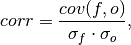
where
 and
and  represent the standard deviation
of the forecast and verification data over the experimental period, respectively.
represent the standard deviation
of the forecast and verification data over the experimental period, respectively.Note
Use metric
_pearson_r_p_value()or_pearson_r_eff_p_value()to get the corresponding p value.- Parameters
forecast – Forecast.
verif – Verification data.
dim – Dimension(s) to perform metric over.
metric_kwargs – see
xskillscore.pearson_r()
Notes
minimum
-1.0
maximum
1.0
perfect
1.0
orientation
positive
See also
Example
>>> HindcastEnsemble.verify(
...     metric="pearson_r",
...     comparison="e2o",
...     alignment="same_verifs",
...     dim=["init"],
... )
<xarray.Dataset>
Dimensions:  (lead: 10)
Coordinates:
  * lead     (lead) int32 1 2 3 4 5 6 7 8 9 10
    skill    <U11 'initialized'
Data variables:
    SST      (lead) float64 0.9272 0.9145 0.9127 0.9319 ... 0.9315 0.9185 0.9112
Attributes:
    prediction_skill_software:     climpred https://climpred.readthedocs.io/
    skill_calculated_by_function:  HindcastEnsemble.verify()
    number_of_initializations:     64
    number_of_members:             10
    alignment:                     same_verifs
    metric:                        pearson_r
    comparison:                    e2o
    dim:                           ['init']
    reference:                     []
Pearson Correlation p value
# Enter any of the below keywords in ``metric=...`` for the compute functions.
In [2]: print(f"Keywords: {metric_aliases['pearson_r_p_value']}")
Keywords: ['pearson_r_p_value', 'p_pval', 'pvalue', 'pval']
- climpred.metrics._pearson_r_p_value(forecast: xarray.Dataset, verif: xarray.Dataset, dim: Optional[Union[str, List[str]]] = None, **metric_kwargs: Any) xarray.Dataset[source]
Probability that forecast and verification data are linearly uncorrelated.
Two-tailed p value associated with the Pearson product-moment correlation coefficient
_pearson_r(), assuming that all samples are independent. Use_pearson_r_eff_p_value()to account for autocorrelation in the forecast and verification data.- Parameters
forecast – Forecast.
verif – Verification data.
dim – Dimension(s) to perform metric over.
metric_kwargs – see
xskillscore.pearson_r_p_value()
Notes
minimum
0.0
maximum
1.0
perfect
1.0
orientation
negative
See also
Example
>>> HindcastEnsemble.verify(
...     metric="pearson_r_p_value",
...     comparison="e2o",
...     alignment="same_verifs",
...     dim="init",
... )
<xarray.Dataset>
Dimensions:  (lead: 10)
Coordinates:
  * lead     (lead) int32 1 2 3 4 5 6 7 8 9 10
    skill    <U11 'initialized'
Data variables:
    SST      (lead) float64 5.779e-23 2.753e-21 4.477e-21 ... 8.7e-22 6.781e-21
Attributes:
    prediction_skill_software:     climpred https://climpred.readthedocs.io/
    skill_calculated_by_function:  HindcastEnsemble.verify()
    number_of_initializations:     64
    number_of_members:             10
    alignment:                     same_verifs
    metric:                        pearson_r_p_value
    comparison:                    e2o
    dim:                           init
    reference:                     []
Effective Sample Size
# Enter any of the below keywords in ``metric=...`` for the compute functions.
In [3]: print(f"Keywords: {metric_aliases['effective_sample_size']}")
Keywords: ['effective_sample_size', 'n_eff', 'eff_n']
- climpred.metrics._effective_sample_size(forecast: xarray.Dataset, verif: xarray.Dataset, dim: Optional[Union[str, List[str]]] = None, **metric_kwargs: Any) xarray.Dataset[source]
Effective sample size for temporally correlated data.
Note
Weights are not included here due to the dependence on temporal autocorrelation.
Note
This metric can only be used for hindcast-type simulations.
The effective sample size extracts the number of independent samples between two time series being correlated. This is derived by assessing the magnitude of the lag-1 autocorrelation coefficient in each of the time series being correlated. A higher autocorrelation induces a lower effective sample size which raises the correlation coefficient for a given p value.
The effective sample size is used in computing the effective p value. See
_pearson_r_eff_p_value()and_spearman_r_eff_p_value().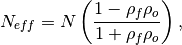
where
 and
and  are the lag-1 autocorrelation
coefficients for the forecast and verification data.
are the lag-1 autocorrelation
coefficients for the forecast and verification data.- Parameters
forecast – Forecast.
verif – Verification data.
dim – Dimension(s) to perform metric over.
metric_kwargs – see
xskillscore.effective_sample_size()
Notes
minimum
0.0
maximum
∞
perfect
N/A
orientation
positive
References
Bretherton et al. [1999]
Example
>>> HindcastEnsemble.verify(
...     metric="effective_sample_size",
...     comparison="e2o",
...     alignment="same_verifs",
...     dim="init",
... )
<xarray.Dataset>
Dimensions:  (lead: 10)
Coordinates:
  * lead     (lead) int32 1 2 3 4 5 6 7 8 9 10
    skill    <U11 'initialized'
Data variables:
    SST      (lead) float64 5.0 4.0 3.0 3.0 3.0 3.0 3.0 3.0 3.0 3.0
Attributes:
    prediction_skill_software:     climpred https://climpred.readthedocs.io/
    skill_calculated_by_function:  HindcastEnsemble.verify()
    number_of_initializations:     64
    number_of_members:             10
    alignment:                     same_verifs
    metric:                        effective_sample_size
    comparison:                    e2o
    dim:                           init
    reference:                     []
Pearson Correlation Effective p value
# Enter any of the below keywords in ``metric=...`` for the compute functions.
In [4]: print(f"Keywords: {metric_aliases['pearson_r_eff_p_value']}")
Keywords: ['pearson_r_eff_p_value', 'p_pval_eff', 'pvalue_eff', 'pval_eff']
- climpred.metrics._pearson_r_eff_p_value(forecast: xarray.Dataset, verif: xarray.Dataset, dim: Optional[Union[str, List[str]]] = None, **metric_kwargs: Any) xarray.Dataset[source]
pearson_r_p_value accounting for autocorrelation.
Note
Weights are not included here due to the dependence on temporal autocorrelation.
Note
This metric can only be used for hindcast-type simulations.
The effective p value is computed by replacing the sample size
 in the
t-statistic with the effective sample size,
in the
t-statistic with the effective sample size,  . The same Pearson
product-moment correlation coefficient
. The same Pearson
product-moment correlation coefficient  is used as when computing the
standard p value.
is used as when computing the
standard p value.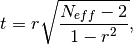
where
is computed via the autocorrelation in the forecast and
verification data.where
and are the lag-1 autocorrelation
coefficients for the forecast and verification data.- Parameters
forecast – Forecast.
verif – Verification data.
dim – Dimension(s) to perform metric over.
metric_kwargs – see
xskillscore.pearson_r_eff_p_value()
Notes
minimum
0.0
maximum
1.0
perfect
1.0
orientation
negative
Example
>>> HindcastEnsemble.verify(
...     metric="pearson_r_eff_p_value",
...     comparison="e2o",
...     alignment="same_verifs",
...     dim="init",
... )
<xarray.Dataset>
Dimensions:  (lead: 10)
Coordinates:
  * lead     (lead) int32 1 2 3 4 5 6 7 8 9 10
    skill    <U11 'initialized'
Data variables:
    SST      (lead) float64 0.02333 0.08552 0.2679 ... 0.2369 0.2588 0.2703
Attributes:
    prediction_skill_software:     climpred https://climpred.readthedocs.io/
    skill_calculated_by_function:  HindcastEnsemble.verify()
    number_of_initializations:     64
    number_of_members:             10
    alignment:                     same_verifs
    metric:                        pearson_r_eff_p_value
    comparison:                    e2o
    dim:                           init
    reference:                     []
References
Bretherton et al. [1999]
Spearman’s Rank Correlation Coefficient
# Enter any of the below keywords in ``metric=...`` for the compute functions.
In [5]: print(f"Keywords: {metric_aliases['spearman_r']}")
Keywords: ['spearman_r', 'sacc', 'sr']
- climpred.metrics._spearman_r(forecast: xarray.Dataset, verif: xarray.Dataset, dim: Optional[Union[str, List[str]]] = None, **metric_kwargs: Any) xarray.Dataset[source]
Spearman’s rank correlation coefficient.

This correlation coefficient is nonparametric and assesses how well the relationship between the forecast and verification data can be described using a monotonic function. It is computed by first ranking the forecasts and verification data, and then correlating those ranks using the
_pearson_r()correlation.This is also known as the anomaly correlation coefficient (ACC) when comparing anomalies, although the Pearson product-moment correlation coefficient
_pearson_r()is typically used when computing the ACC.Note
Use metric
_spearman_r_p_value()or_spearman_r_eff_p_value`()to get the corresponding p value.- Parameters
forecast – Forecast.
verif – Verification data.
dim – Dimension(s) to perform metric over.
metric_kwargs – see
xskillscore.spearman_r()
Notes
minimum
-1.0
maximum
1.0
perfect
1.0
orientation
positive
See also
Example
>>> HindcastEnsemble.verify(
...     metric="spearman_r",
...     comparison="e2o",
...     alignment="same_verifs",
...     dim="init",
... )
<xarray.Dataset>
Dimensions:  (lead: 10)
Coordinates:
  * lead     (lead) int32 1 2 3 4 5 6 7 8 9 10
    skill    <U11 'initialized'
Data variables:
    SST      (lead) float64 0.9336 0.9311 0.9293 0.9474 ... 0.9465 0.9346 0.9328
Attributes:
    prediction_skill_software:     climpred https://climpred.readthedocs.io/
    skill_calculated_by_function:  HindcastEnsemble.verify()
    number_of_initializations:     64
    number_of_members:             10
    alignment:                     same_verifs
    metric:                        spearman_r
    comparison:                    e2o
    dim:                           init
    reference:                     []
Spearman’s Rank Correlation Coefficient p value
# Enter any of the below keywords in ``metric=...`` for the compute functions.
In [6]: print(f"Keywords: {metric_aliases['spearman_r_p_value']}")
Keywords: ['spearman_r_p_value', 's_pval', 'spvalue', 'spval']
- climpred.metrics._spearman_r_p_value(forecast: xarray.Dataset, verif: xarray.Dataset, dim: Optional[Union[str, List[str]]] = None, **metric_kwargs: Any) xarray.Dataset[source]
Probability that forecast and verification data are monotonically uncorrelated.
Two-tailed p value associated with the Spearman’s rank correlation coefficient
_spearman_r(), assuming that all samples are independent. Use_spearman_r_eff_p_value()to account for autocorrelation in the forecast and verification data.- Parameters
forecast – Forecast.
verif – Verification data.
dim – Dimension(s) to perform metric over.
metric_kwargs – see
xskillscore.spearman_r_p_value()
Notes
minimum
0.0
maximum
1.0
perfect
1.0
orientation
negative
See also
Example
>>> HindcastEnsemble.verify(
...     metric="spearman_r_p_value",
...     comparison="e2o",
...     alignment="same_verifs",
...     dim="init",
... )
<xarray.Dataset>
Dimensions:  (lead: 10)
Coordinates:
  * lead     (lead) int32 1 2 3 4 5 6 7 8 9 10
    skill    <U11 'initialized'
Data variables:
    SST      (lead) float64 6.248e-24 1.515e-23 ... 4.288e-24 8.254e-24
Attributes:
    prediction_skill_software:     climpred https://climpred.readthedocs.io/
    skill_calculated_by_function:  HindcastEnsemble.verify()
    number_of_initializations:     64
    number_of_members:             10
    alignment:                     same_verifs
    metric:                        spearman_r_p_value
    comparison:                    e2o
    dim:                           init
    reference:                     []
Spearman’s Rank Correlation Effective p value
# Enter any of the below keywords in ``metric=...`` for the compute functions.
In [7]: print(f"Keywords: {metric_aliases['spearman_r_eff_p_value']}")
Keywords: ['spearman_r_eff_p_value', 's_pval_eff', 'spvalue_eff', 'spval_eff']
- climpred.metrics._spearman_r_eff_p_value(forecast: xarray.Dataset, verif: xarray.Dataset, dim: Optional[Union[str, List[str]]] = None, **metric_kwargs: Any) xarray.Dataset[source]
_spearman_r_p_value accounting for autocorrelation.
Note
Weights are not included here due to the dependence on temporal autocorrelation.
Note
This metric can only be used for hindcast-type simulations.
The effective p value is computed by replacing the sample size
in the
t-statistic with the effective sample size, . The same Spearman’s
rank correlation coefficient is used as when computing the standard p
value.where
is computed via the autocorrelation in the forecast and
verification data.where
and are the lag-1 autocorrelation
coefficients for the forecast and verification data.- Parameters
forecast – Forecast.
verif – Verification data.
dim – Dimension(s) to perform metric over.
metric_kwargs – see
xskillscore.spearman_r_eff_p_value()
Notes
minimum
0.0
maximum
1.0
perfect
1.0
orientation
negative
References
Bretherton et al. [1999]
Example
>>> HindcastEnsemble.verify(
...     metric="spearman_r_eff_p_value",
...     comparison="e2o",
...     alignment="same_verifs",
...     dim="init",
... )
<xarray.Dataset>
Dimensions:  (lead: 10)
Coordinates:
  * lead     (lead) int32 1 2 3 4 5 6 7 8 9 10
    skill    <U11 'initialized'
Data variables:
    SST      (lead) float64 0.02034 0.0689 0.2408 ... 0.2092 0.2315 0.2347
Attributes:
    prediction_skill_software:     climpred https://climpred.readthedocs.io/
    skill_calculated_by_function:  HindcastEnsemble.verify()
    number_of_initializations:     64
    number_of_members:             10
    alignment:                     same_verifs
    metric:                        spearman_r_eff_p_value
    comparison:                    e2o
    dim:                           init
    reference:                     []
Distance Metrics
This class of metrics simply measures the distance (or difference) between forecasted values and observed values.
Mean Squared Error (MSE)
# Enter any of the below keywords in ``metric=...`` for the compute functions.
In [8]: print(f"Keywords: {metric_aliases['mse']}")
Keywords: ['mse']
- climpred.metrics._mse(forecast: xarray.Dataset, verif: xarray.Dataset, dim: Optional[Union[str, List[str]]] = None, **metric_kwargs: Any) xarray.Dataset[source]
Mean Sqaure Error (MSE).
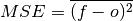
The average of the squared difference between forecasts and verification data. This incorporates both the variance and bias of the estimator. Because the error is squared, it is more sensitive to large forecast errors than
mae, and thus a more conservative metric. For example, a single error of 2°C counts the same as two 1°C errors when usingmae. On the other hand, the 2°C error counts double formse. See Jolliffe and Stephenson, 2011.- Parameters
forecast – Forecast.
verif – Verification data.
dim – Dimension(s) to perform metric over.
metric_kwargs – see
xskillscore.mse()
Notes
minimum
0.0
maximum
∞
perfect
0.0
orientation
negative
See also
References
Jolliffe and Stephenson [2011]
Example
>>> HindcastEnsemble.verify(
...     metric="mse", comparison="e2o", alignment="same_verifs", dim="init"
... )
<xarray.Dataset>
Dimensions:  (lead: 10)
Coordinates:
  * lead     (lead) int32 1 2 3 4 5 6 7 8 9 10
    skill    <U11 'initialized'
Data variables:
    SST      (lead) float64 0.006202 0.006536 0.007771 ... 0.02417 0.02769
Attributes:
    prediction_skill_software:     climpred https://climpred.readthedocs.io/
    skill_calculated_by_function:  HindcastEnsemble.verify()
    number_of_initializations:     64
    number_of_members:             10
    alignment:                     same_verifs
    metric:                        mse
    comparison:                    e2o
    dim:                           init
    reference:                     []
Root Mean Square Error (RMSE)
# Enter any of the below keywords in ``metric=...`` for the compute functions.
In [9]: print(f"Keywords: {metric_aliases['rmse']}")
Keywords: ['rmse']
- climpred.metrics._rmse(forecast: xarray.Dataset, verif: xarray.Dataset, dim: Optional[Union[str, List[str]]] = None, **metric_kwargs: Any) xarray.Dataset[source]
Root Mean Sqaure Error (RMSE).
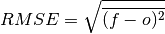
The square root of the average of the squared differences between forecasts and verification data.
- Parameters
forecast – Forecast.
verif – Verification data.
dim – Dimension(s) to perform metric over.
metric_kwargs – see
xskillscore.rmse()
Notes
minimum
0.0
maximum
∞
perfect
0.0
orientation
negative
See also
Example
>>> HindcastEnsemble.verify(
...     metric="rmse", comparison="e2o", alignment="same_verifs", dim="init"
... )
<xarray.Dataset>
Dimensions:  (lead: 10)
Coordinates:
  * lead     (lead) int32 1 2 3 4 5 6 7 8 9 10
    skill    <U11 'initialized'
Data variables:
    SST      (lead) float64 0.07875 0.08085 0.08815 ... 0.1371 0.1555 0.1664
Attributes:
    prediction_skill_software:     climpred https://climpred.readthedocs.io/
    skill_calculated_by_function:  HindcastEnsemble.verify()
    number_of_initializations:     64
    number_of_members:             10
    alignment:                     same_verifs
    metric:                        rmse
    comparison:                    e2o
    dim:                           init
    reference:                     []
Mean Absolute Error (MAE)
# Enter any of the below keywords in ``metric=...`` for the compute functions.
In [10]: print(f"Keywords: {metric_aliases['mae']}")
Keywords: ['mae']
- climpred.metrics._mae(forecast: xarray.Dataset, verif: xarray.Dataset, dim: Optional[Union[str, List[str]]] = None, **metric_kwargs: Any) xarray.Dataset[source]
Mean Absolute Error (MAE).
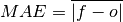
The average of the absolute differences between forecasts and verification data. A more robust measure of forecast accuracy than
msewhich is sensitive to large outlier forecast errors.- Parameters
forecast – Forecast.
verif – Verification data.
dim – Dimension(s) to perform metric over.
metric_kwargs – see
xskillscore.mae()
Notes
minimum
0.0
maximum
∞
perfect
0.0
orientation
negative
See also
References
Jolliffe and Stephenson [2011]
Example
>>> HindcastEnsemble.verify(
...     metric="mae", comparison="e2o", alignment="same_verifs", dim="init"
... )
<xarray.Dataset>
Dimensions:  (lead: 10)
Coordinates:
  * lead     (lead) int32 1 2 3 4 5 6 7 8 9 10
    skill    <U11 'initialized'
Data variables:
    SST      (lead) float64 0.06484 0.06684 0.07407 ... 0.1193 0.1361 0.1462
Attributes:
    prediction_skill_software:     climpred https://climpred.readthedocs.io/
    skill_calculated_by_function:  HindcastEnsemble.verify()
    number_of_initializations:     64
    number_of_members:             10
    alignment:                     same_verifs
    metric:                        mae
    comparison:                    e2o
    dim:                           init
    reference:                     []
Median Absolute Error
# Enter any of the below keywords in ``metric=...`` for the compute functions.
In [11]: print(f"Keywords: {metric_aliases['median_absolute_error']}")
Keywords: ['median_absolute_error']
- climpred.metrics._median_absolute_error(forecast: xarray.Dataset, verif: xarray.Dataset, dim: Optional[Union[str, List[str]]] = None, **metric_kwargs: Any) xarray.Dataset[source]
Median Absolute Error.
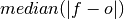
The median of the absolute differences between forecasts and verification data. Applying the median function to absolute error makes it more robust to outliers.
- Parameters
forecast – Forecast.
verif – Verification data.
dim – Dimension(s) to perform metric over.
metric_kwargs – see
xskillscore.median_absolute_error()
Notes
minimum
0.0
maximum
∞
perfect
0.0
orientation
negative
See also
Example
>>> HindcastEnsemble.verify(
...     metric="median_absolute_error",
...     comparison="e2o",
...     alignment="same_verifs",
...     dim="init",
... )
<xarray.Dataset>
Dimensions:  (lead: 10)
Coordinates:
  * lead     (lead) int32 1 2 3 4 5 6 7 8 9 10
    skill    <U11 'initialized'
Data variables:
    SST      (lead) float64 0.06077 0.06556 0.06368 ... 0.1131 0.142 0.1466
Attributes:
    prediction_skill_software:     climpred https://climpred.readthedocs.io/
    skill_calculated_by_function:  HindcastEnsemble.verify()
    number_of_initializations:     64
    number_of_members:             10
    alignment:                     same_verifs
    metric:                        median_absolute_error
    comparison:                    e2o
    dim:                           init
    reference:                     []
Spread
# Enter any of the below keywords in ``metric=...`` for the compute functions.
In [12]: print(f"Keywords: {metric_aliases['spread']}")
Keywords: ['spread']
- climpred.metrics._spread(forecast: xarray.Dataset, verif: xarray.Dataset, dim: Optional[Union[str, List[str]]] = None, **metric_kwargs: Any) xarray.Dataset[source]
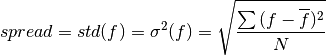
Ensemble spread taking the standard deviation over the member dimension.
- Parameters
forecast – Forecast.
verif – Verification data (not used).
dim – Dimension(s) to perform metric over.
metric_kwargs – see
std()
Notes
minimum
0.0
maximum
∞
perfect
obs.std()
orientation
negative
Example
>>> HindcastEnsemble.verify(
...     metric="spread",
...     comparison="m2o",
...     alignment="same_verifs",
...     dim=["member", "init"],
... )
<xarray.Dataset>
Dimensions:  (lead: 10)
Coordinates:
  * lead     (lead) int32 1 2 3 4 5 6 7 8 9 10
    skill    <U11 'initialized'
Data variables:
    SST      (lead) float64 0.1468 0.1738 0.1922 0.2096 ... 0.2142 0.2178 0.2098
Attributes:
    prediction_skill_software:     climpred https://climpred.readthedocs.io/
    skill_calculated_by_function:  HindcastEnsemble.verify()
    number_of_initializations:     64
    number_of_members:             10
    alignment:                     same_verifs
    metric:                        spread
    comparison:                    m2o
    dim:                           ['member', 'init']
    reference:                     []
Multiplicative bias
# Enter any of the below keywords in ``metric=...`` for the compute functions.
In [13]: print(f"Keywords: {metric_aliases['mul_bias']}")
Keywords: ['mul_bias', 'm_b', 'multiplicative_bias']
- climpred.metrics._mul_bias(forecast: xarray.Dataset, verif: xarray.Dataset, dim: Optional[Union[str, List[str]]] = None, **metric_kwargs: Any) xarray.Dataset[source]
Multiplicative bias.

- Parameters
forecast – Forecast.
verif – Verification data.
dim – Dimension(s) to perform metric over
metric_kwargs – see xarray.mean
Notes
minimum
-∞
maximum
∞
perfect
1.0
orientation
None
Example
>>> HindcastEnsemble.verify(
...     metric="multiplicative_bias",
...     comparison="e2o",
...     alignment="same_verifs",
...     dim="init",
... )
<xarray.Dataset>
Dimensions:  (lead: 10)
Coordinates:
  * lead     (lead) int32 1 2 3 4 5 6 7 8 9 10
    skill    <U11 'initialized'
Data variables:
    SST      (lead) float64 0.719 0.9991 1.072 1.434 ... 1.854 2.128 2.325 2.467
Attributes:
    prediction_skill_software:     climpred https://climpred.readthedocs.io/
    skill_calculated_by_function:  HindcastEnsemble.verify()
    number_of_initializations:     64
    number_of_members:             10
    alignment:                     same_verifs
    metric:                        mul_bias
    comparison:                    e2o
    dim:                           init
    reference:                     []
Normalized Distance Metrics
Distance metrics like mse can be normalized to 1. The normalization factor
depends on the comparison type choosen. For example, the distance between an ensemble
member and the ensemble mean is half the distance of an ensemble member with other
ensemble members. See _get_norm_factor().
Normalized Mean Square Error (NMSE)
# Enter any of the below keywords in ``metric=...`` for the compute functions.
In [14]: print(f"Keywords: {metric_aliases['nmse']}")
Keywords: ['nmse', 'nev']
- climpred.metrics._nmse(forecast: xarray.Dataset, verif: xarray.Dataset, dim: Optional[Union[str, List[str]]] = None, **metric_kwargs: Any) xarray.Dataset[source]
Compte Normalized MSE (NMSE), also known as Normalized Ensemble Variance (NEV).
Mean Square Error (
mse) normalized by the variance of the verification data.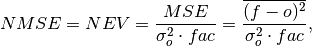
where
 is 1 when using comparisons involving the ensemble mean (
m2e,e2c,e2o) and 2 when using comparisons involving individual ensemble members (m2c,m2m,m2o). See_get_norm_factor().Note
climpreduses a single-valued internal reference forecast for the NMSE, in the terminology of Murphy [1988]. I.e., we use a single climatological variance of the verification data within the experimental window for normalizing MSE.- Parameters
forecast – Forecast.
verif – Verification data.
dim – Dimension(s) to perform metric over.
comparison – Name comparison needed for normalization factor fac, see
_get_norm_factor()(Handled internally by the compute functions)metric_kwargs – see
xskillscore.mse()
Notes
minimum
0.0
maximum
∞
perfect
0.0
orientation
negative
better than climatology
0.0 - 1.0
worse than climatology
> 1.0
References
Griffies and Bryan [1997]
Example
>>> HindcastEnsemble.verify(
...     metric="nmse", comparison="e2o", alignment="same_verifs", dim="init"
... )
<xarray.Dataset>
Dimensions:  (lead: 10)
Coordinates:
  * lead     (lead) int32 1 2 3 4 5 6 7 8 9 10
    skill    <U11 'initialized'
Data variables:
    SST      (lead) float64 0.1732 0.1825 0.217 0.2309 ... 0.5247 0.6749 0.7732
Attributes:
    prediction_skill_software:     climpred https://climpred.readthedocs.io/
    skill_calculated_by_function:  HindcastEnsemble.verify()
    number_of_initializations:     64
    number_of_members:             10
    alignment:                     same_verifs
    metric:                        nmse
    comparison:                    e2o
    dim:                           init
    reference:                     []
Normalized Mean Absolute Error (NMAE)
# Enter any of the below keywords in ``metric=...`` for the compute functions.
In [15]: print(f"Keywords: {metric_aliases['nmae']}")
Keywords: ['nmae']
- climpred.metrics._nmae(forecast: xarray.Dataset, verif: xarray.Dataset, dim: Optional[Union[str, List[str]]] = None, **metric_kwargs: Any) xarray.Dataset[source]
Compute Normalized Mean Absolute Error (NMAE).
Mean Absolute Error (
mae) normalized by the standard deviation of the verification data.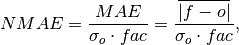
where
is 1 when using comparisons involving the ensemble mean (m2e,e2c,e2o) and 2 when using comparisons involving individual ensemble members (m2c,m2m,m2o). See_get_norm_factor().Note
climpreduses a single-valued internal reference forecast for the NMAE, in the terminology of Murphy [1988]. I.e., we use a single climatological standard deviation of the verification data within the experimental window for normalizing MAE.- Parameters
forecast – Forecast.
verif – Verification data.
dim – Dimension(s) to perform metric over.
comparison – Name comparison needed for normalization factor fac, see
_get_norm_factor()(Handled internally by the compute functions)metric_kwargs – see
xskillscore.mae()
Notes
minimum
0.0
maximum
∞
perfect
0.0
orientation
negative
better than climatology
0.0 - 1.0
worse than climatology
> 1.0
References
Example
>>> HindcastEnsemble.verify(
...     metric="nmae", comparison="e2o", alignment="same_verifs", dim="init"
... )
<xarray.Dataset>
Dimensions:  (lead: 10)
Coordinates:
  * lead     (lead) int32 1 2 3 4 5 6 7 8 9 10
    skill    <U11 'initialized'
Data variables:
    SST      (lead) float64 0.3426 0.3532 0.3914 0.3898 ... 0.6303 0.7194 0.7726
Attributes:
    prediction_skill_software:     climpred https://climpred.readthedocs.io/
    skill_calculated_by_function:  HindcastEnsemble.verify()
    number_of_initializations:     64
    number_of_members:             10
    alignment:                     same_verifs
    metric:                        nmae
    comparison:                    e2o
    dim:                           init
    reference:                     []
Normalized Root Mean Square Error (NRMSE)
# Enter any of the below keywords in ``metric=...`` for the compute functions.
In [16]: print(f"Keywords: {metric_aliases['nrmse']}")
Keywords: ['nrmse']
- climpred.metrics._nrmse(forecast: xarray.Dataset, verif: xarray.Dataset, dim: Optional[Union[str, List[str]]] = None, **metric_kwargs: Any) xarray.Dataset[source]
Compute Normalized Root Mean Square Error (NRMSE).
Root Mean Square Error (
rmse) normalized by the standard deviation of the verification data.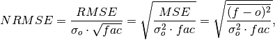
where
is 1 when using comparisons involving the ensemble mean (m2e,e2c,e2o) and 2 when using comparisons involving individual ensemble members (m2c,m2m,m2o). See_get_norm_factor().Note
climpreduses a single-valued internal reference forecast for the NRMSE, in the terminology of Murphy [1988]. I.e., we use a single climatological variance of the verification data within the experimental window for normalizing RMSE.- Parameters
forecast – Forecast.
verif – Verification data.
dim – Dimension(s) to perform metric over.
comparison – Name comparison needed for normalization factor fac, see
_get_norm_factor()(Handled internally by the compute functions)metric_kwargs – see
xskillscore.rmse()
Notes
minimum
0.0
maximum
∞
perfect
0.0
orientation
negative
better than climatology
0.0 - 1.0
worse than climatology
> 1.0
References
Example
>>> HindcastEnsemble.verify(
...     metric="nrmse", comparison="e2o", alignment="same_verifs", dim="init"
... )
<xarray.Dataset>
Dimensions:  (lead: 10)
Coordinates:
  * lead     (lead) int32 1 2 3 4 5 6 7 8 9 10
    skill    <U11 'initialized'
Data variables:
    SST      (lead) float64 0.4161 0.4272 0.4658 0.4806 ... 0.7244 0.8215 0.8793
Attributes:
    prediction_skill_software:     climpred https://climpred.readthedocs.io/
    skill_calculated_by_function:  HindcastEnsemble.verify()
    number_of_initializations:     64
    number_of_members:             10
    alignment:                     same_verifs
    metric:                        nrmse
    comparison:                    e2o
    dim:                           init
    reference:                     []
Mean Square Error Skill Score (MSESS)
# Enter any of the below keywords in ``metric=...`` for the compute functions.
In [17]: print(f"Keywords: {metric_aliases['msess']}")
Keywords: ['msess', 'ppp', 'msss']
- climpred.metrics._msess(forecast: xarray.Dataset, verif: xarray.Dataset, dim: Optional[Union[str, List[str]]] = None, **metric_kwargs: Any) xarray.Dataset[source]
Mean Squared Error Skill Score (MSESS).
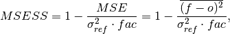
where
is 1 when using comparisons involving the ensemble mean (m2e,e2c,e2o) and 2 when using comparisons involving individual ensemble members (m2c,m2m,m2o). See_get_norm_factor().This skill score can be intepreted as a percentage improvement in accuracy. I.e., it can be multiplied by 100%.
Note
climpreduses a single-valued internal reference forecast for the MSSS, in the terminology of Murphy [1988]. I.e., we use a single climatological variance of the verification data within the experimental window for normalizing MSE.- Parameters
forecast – Forecast.
verif – Verification data.
dim – Dimension(s) to perform metric over.
comparison – Name comparison needed for normalization factor fac, see
_get_norm_factor()(Handled internally by the compute functions)metric_kwargs – see
xskillscore.mse()
Notes
minimum
-∞
maximum
1.0
perfect
1.0
orientation
positive
better than climatology
> 0.0
equal to climatology
0.0
worse than climatology
< 0.0
References
Example
>>> HindcastEnsemble.verify(
...     metric="msess", comparison="e2o", alignment="same_verifs", dim="init"
... )
<xarray.Dataset>
Dimensions:  (lead: 10)
Coordinates:
  * lead     (lead) int32 1 2 3 4 5 6 7 8 9 10
    skill    <U11 'initialized'
Data variables:
    SST      (lead) float64 0.8268 0.8175 0.783 0.7691 ... 0.4753 0.3251 0.2268
Attributes:
    prediction_skill_software:     climpred https://climpred.readthedocs.io/
    skill_calculated_by_function:  HindcastEnsemble.verify()
    number_of_initializations:     64
    number_of_members:             10
    alignment:                     same_verifs
    metric:                        msess
    comparison:                    e2o
    dim:                           init
    reference:                     []
Mean Absolute Percentage Error (MAPE)
# Enter any of the below keywords in ``metric=...`` for the compute functions.
In [18]: print(f"Keywords: {metric_aliases['mape']}")
Keywords: ['mape']
- climpred.metrics._mape(forecast: xarray.Dataset, verif: xarray.Dataset, dim: Optional[Union[str, List[str]]] = None, **metric_kwargs: Any) xarray.Dataset[source]
Mean Absolute Percentage Error (MAPE).
Mean absolute error (
mae) expressed as the fractional error relative to the verification data.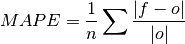
- Parameters
forecast – Forecast.
verif – Verification data.
dim – Dimension(s) to perform metric over.
metric_kwargs – see
xskillscore.mape()
Notes
minimum
0.0
maximum
∞
perfect
0.0
orientation
negative
See also
Example
>>> HindcastEnsemble.verify(
...     metric="mape", comparison="e2o", alignment="same_verifs", dim="init"
... )
<xarray.Dataset>
Dimensions:  (lead: 10)
Coordinates:
  * lead     (lead) int32 1 2 3 4 5 6 7 8 9 10
    skill    <U11 'initialized'
Data variables:
    SST      (lead) float64 1.536 1.21 1.421 1.149 ... 1.078 1.369 1.833 1.245
Attributes:
    prediction_skill_software:     climpred https://climpred.readthedocs.io/
    skill_calculated_by_function:  HindcastEnsemble.verify()
    number_of_initializations:     64
    number_of_members:             10
    alignment:                     same_verifs
    metric:                        mape
    comparison:                    e2o
    dim:                           init
    reference:                     []
Symmetric Mean Absolute Percentage Error (sMAPE)
# Enter any of the below keywords in ``metric=...`` for the compute functions.
In [19]: print(f"Keywords: {metric_aliases['smape']}")
Keywords: ['smape']
- climpred.metrics._smape(forecast: xarray.Dataset, verif: xarray.Dataset, dim: Optional[Union[str, List[str]]] = None, **metric_kwargs: Any) xarray.Dataset[source]
Symmetric Mean Absolute Percentage Error (sMAPE).
Similar to the Mean Absolute Percentage Error (
mape), but sums the forecast and observation mean in the denominator.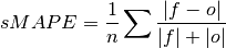
- Parameters
forecast – Forecast.
verif – Verification data.
dim – Dimension(s) to perform metric over.
metric_kwargs – see
xskillscore.smape()
Notes
minimum
0.0
maximum
1.0
perfect
0.0
orientation
negative
See also
Example
>>> HindcastEnsemble.verify(
...     metric="smape", comparison="e2o", alignment="same_verifs", dim="init"
... )
<xarray.Dataset>
Dimensions:  (lead: 10)
Coordinates:
  * lead     (lead) int32 1 2 3 4 5 6 7 8 9 10
    skill    <U11 'initialized'
Data variables:
    SST      (lead) float64 0.3801 0.3906 0.4044 0.3819 ... 0.4822 0.5054 0.5295
Attributes:
    prediction_skill_software:     climpred https://climpred.readthedocs.io/
    skill_calculated_by_function:  HindcastEnsemble.verify()
    number_of_initializations:     64
    number_of_members:             10
    alignment:                     same_verifs
    metric:                        smape
    comparison:                    e2o
    dim:                           init
    reference:                     []
Unbiased Anomaly Correlation Coefficient (uACC)
# Enter any of the below keywords in ``metric=...`` for the compute functions.
In [20]: print(f"Keywords: {metric_aliases['uacc']}")
Keywords: ['uacc']
- climpred.metrics._uacc(forecast: xarray.Dataset, verif: xarray.Dataset, dim: Optional[Union[str, List[str]]] = None, **metric_kwargs: Any) xarray.Dataset[source]
Bushuk’s unbiased Anomaly Correlation Coefficient (uACC).
This is typically used in perfect model studies. Because the perfect model Anomaly Correlation Coefficient (ACC) is strongly state dependent, a standard ACC (e.g. one computed using
_pearson_r()) will be highly sensitive to the set of start dates chosen for the perfect model study. The Mean Square Skill Score (MESSS) can be related directly to the ACC asMESSS = ACC^(2)(see Murphy [1988] and Bushuk et al. [2018]), so the unbiased ACC can be derived asuACC = sqrt(MESSS).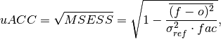
where
is 1 when using comparisons involving the ensemble mean (m2e,e2c,e2o) and 2 when using comparisons involving individual ensemble members (m2c,m2m,m2o). See_get_norm_factor().Note
Because of the square root involved, any negative
MSESSvalues are automatically converted to NaNs.- Parameters
forecast – Forecast.
verif – Verification data.
dim – Dimension(s) to perform metric over.
comparison – Name comparison needed for normalization factor
fac, see_get_norm_factor()(Handled internally by the compute functions)metric_kwargs – see
xskillscore.mse()
Notes
minimum
0.0
maximum
1.0
perfect
1.0
orientation
positive
better than climatology
> 0.0
equal to climatology
0.0
References
Example
>>> HindcastEnsemble.verify(
...     metric="uacc", comparison="e2o", alignment="same_verifs", dim="init"
... )
<xarray.Dataset>
Dimensions:  (lead: 10)
Coordinates:
  * lead     (lead) int32 1 2 3 4 5 6 7 8 9 10
    skill    <U11 'initialized'
Data variables:
    SST      (lead) float64 0.9093 0.9041 0.8849 0.877 ... 0.6894 0.5702 0.4763
Attributes:
    prediction_skill_software:     climpred https://climpred.readthedocs.io/
    skill_calculated_by_function:  HindcastEnsemble.verify()
    number_of_initializations:     64
    number_of_members:             10
    alignment:                     same_verifs
    metric:                        uacc
    comparison:                    e2o
    dim:                           init
    reference:                     []
Murphy Decomposition Metrics
Metrics derived in [Murphy, 1988] which decompose the MSESS into a correlation term,
a conditional bias term, and an unconditional bias term. See
https://www-miklip.dkrz.de/about/murcss/ for a walk through of the decomposition.
Standard Ratio
# Enter any of the below keywords in ``metric=...`` for the compute functions.
In [21]: print(f"Keywords: {metric_aliases['std_ratio']}")
Keywords: ['std_ratio']
- climpred.metrics._std_ratio(forecast: xarray.Dataset, verif: xarray.Dataset, dim: Optional[Union[str, List[str]]] = None, **metric_kwargs: Any) xarray.Dataset[source]
Ratio of standard deviations of the forecast over the verification data.
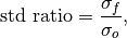
where
and are the standard deviations of the
forecast and the verification data over the experimental period, respectively.- Parameters
forecast – Forecast.
verif – Verification data.
dim – Dimension(s) to perform metric over.
metric_kwargs – see xarray.std
Notes
minimum
0.0
maximum
∞
perfect
1.0
orientation
N/A
References
Example
>>> HindcastEnsemble.verify(
...     metric="std_ratio",
...     comparison="e2o",
...     alignment="same_verifs",
...     dim="init",
... )
<xarray.Dataset>
Dimensions:  (lead: 10)
Coordinates:
  * lead     (lead) int32 1 2 3 4 5 6 7 8 9 10
    skill    <U11 'initialized'
Data variables:
    SST      (lead) float64 0.7567 0.8801 0.9726 1.055 ... 1.075 1.094 1.055
Attributes:
    prediction_skill_software:     climpred https://climpred.readthedocs.io/
    skill_calculated_by_function:  HindcastEnsemble.verify()
    number_of_initializations:     64
    number_of_members:             10
    alignment:                     same_verifs
    metric:                        std_ratio
    comparison:                    e2o
    dim:                           init
    reference:                     []
Conditional Bias
# Enter any of the below keywords in ``metric=...`` for the compute functions.
In [22]: print(f"Keywords: {metric_aliases['conditional_bias']}")
Keywords: ['conditional_bias', 'c_b', 'cond_bias']
- climpred.metrics._conditional_bias(forecast: xarray.Dataset, verif: xarray.Dataset, dim: Optional[Union[str, List[str]]] = None, **metric_kwargs: Any) xarray.Dataset[source]
Conditional bias between forecast and verification data.
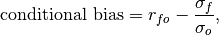
where
and are the standard deviations of the
forecast and verification data over the experimental period, respectively.- Parameters
forecast – Forecast.
verif – Verification data.
dim – Dimension(s) to perform metric over.
metric_kwargs – see
xskillscore.pearson_r()andstd()
Notes
minimum
-∞
maximum
1.0
perfect
0.0
orientation
negative
References
https://www-miklip.dkrz.de/about/murcss/
Example
>>> HindcastEnsemble.verify(
...     metric="conditional_bias",
...     comparison="e2o",
...     alignment="same_verifs",
...     dim="init",
... )
<xarray.Dataset>
Dimensions:  (lead: 10)
Coordinates:
  * lead     (lead) int32 1 2 3 4 5 6 7 8 9 10
    skill    <U11 'initialized'
Data variables:
    SST      (lead) float64 0.1705 0.03435 -0.05988 ... -0.1436 -0.175 -0.1434
Attributes:
    prediction_skill_software:     climpred https://climpred.readthedocs.io/
    skill_calculated_by_function:  HindcastEnsemble.verify()
    number_of_initializations:     64
    number_of_members:             10
    alignment:                     same_verifs
    metric:                        conditional_bias
    comparison:                    e2o
    dim:                           init
    reference:                     []
Unconditional Bias
# Enter any of the below keywords in ``metric=...`` for the compute functions.
In [23]: print(f"Keywords: {metric_aliases['unconditional_bias']}")
Keywords: ['unconditional_bias', 'u_b', 'a_b', 'bias', 'additive_bias']
Simple bias of the forecast minus the observations.
- climpred.metrics._unconditional_bias(forecast: xarray.Dataset, verif: xarray.Dataset, dim: Optional[Union[str, List[str]]] = None, **metric_kwargs: Any) xarray.Dataset[source]
Unconditional additive bias.

- Parameters
forecast – Forecast.
verif – Verification data.
dim – Dimension(s) to perform metric over
metric_kwargs – see xarray.mean
Notes
minimum
-∞
maximum
∞
perfect
0.0
orientation
negative
References
Example
>>> HindcastEnsemble.verify(
...     metric="unconditional_bias",
...     comparison="e2o",
...     alignment="same_verifs",
...     dim="init",
... )
<xarray.Dataset>
Dimensions:  (lead: 10)
Coordinates:
  * lead     (lead) int32 1 2 3 4 5 6 7 8 9 10
    skill    <U11 'initialized'
Data variables:
    SST      (lead) float64 -0.01158 -0.02512 -0.0408 ... -0.1322 -0.1445
Attributes:
    prediction_skill_software:     climpred https://climpred.readthedocs.io/
    skill_calculated_by_function:  HindcastEnsemble.verify()
    number_of_initializations:     64
    number_of_members:             10
    alignment:                     same_verifs
    metric:                        unconditional_bias
    comparison:                    e2o
    dim:                           init
    reference:                     []
Conditional bias is removed by
HindcastEnsemble.remove_bias().>>> HindcastEnsemble = HindcastEnsemble.remove_bias(alignment="same_verifs") >>> HindcastEnsemble.verify( ... metric="unconditional_bias", ... comparison="e2o", ... alignment="same_verifs", ... dim="init", ... ) <xarray.Dataset> Dimensions: (lead: 10) Coordinates: * lead (lead) int32 1 2 3 4 5 6 7 8 9 10 skill <U11 'initialized' Data variables: SST (lead) float64 3.203e-18 -1.068e-18 ... 2.882e-17 -2.776e-17 Attributes: prediction_skill_software: climpred https://climpred.readthedocs.io/ skill_calculated_by_function: HindcastEnsemble.verify() number_of_initializations: 64 number_of_members: 10 alignment: same_verifs metric: unconditional_bias comparison: e2o dim: init reference: []
Bias Slope
# Enter any of the below keywords in ``metric=...`` for the compute functions.
In [24]: print(f"Keywords: {metric_aliases['bias_slope']}")
Keywords: ['bias_slope']
- climpred.metrics._bias_slope(forecast: xarray.Dataset, verif: xarray.Dataset, dim: Optional[Union[str, List[str]]] = None, **metric_kwargs: Any) xarray.Dataset[source]
Bias slope between verification data and forecast standard deviations.
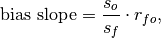
where
 is the Pearson product-moment correlation between the forecast
and the verification data and
is the Pearson product-moment correlation between the forecast
and the verification data and  and
and  are the standard
deviations of the verification data and forecast over the experimental period,
respectively.
are the standard
deviations of the verification data and forecast over the experimental period,
respectively.- Parameters
forecast – Forecast.
verif – Verification data.
dim – Dimension(s) to perform metric over.
metric_kwargs – see
xskillscore.pearson_r()andstd()
Notes
minimum
0.0
maximum
∞
perfect
1.0
orientation
negative
References
https://www-miklip.dkrz.de/about/murcss/
Example
>>> HindcastEnsemble.verify(
...     metric="bias_slope",
...     comparison="e2o",
...     alignment="same_verifs",
...     dim="init",
... )
<xarray.Dataset>
Dimensions:  (lead: 10)
Coordinates:
  * lead     (lead) int32 1 2 3 4 5 6 7 8 9 10
    skill    <U11 'initialized'
Data variables:
    SST      (lead) float64 0.7016 0.8049 0.8877 0.9836 ... 1.002 1.004 0.961
Attributes:
    prediction_skill_software:     climpred https://climpred.readthedocs.io/
    skill_calculated_by_function:  HindcastEnsemble.verify()
    number_of_initializations:     64
    number_of_members:             10
    alignment:                     same_verifs
    metric:                        bias_slope
    comparison:                    e2o
    dim:                           init
    reference:                     []
Murphy’s Mean Square Error Skill Score
# Enter any of the below keywords in ``metric=...`` for the compute functions.
In [25]: print(f"Keywords: {metric_aliases['msess_murphy']}")
Keywords: ['msess_murphy', 'msss_murphy']
- climpred.metrics._msess_murphy(forecast: xarray.Dataset, verif: xarray.Dataset, dim: Optional[Union[str, List[str]]] = None, **metric_kwargs: Any) xarray.Dataset[source]
Murphy’s Mean Square Error Skill Score (MSESS).
![MSESS_{Murphy} = r_{fo}^2 - [\text{conditional bias}]^2 -\
[\frac{\text{(unconditional) bias}}{\sigma_o}]^2,](_images/math/97a8a3bd5f45b4e7aebe33441fd0097a78a5c6e4.png)
where
 represents the Pearson product-moment correlation
coefficient between the forecast and verification data and
represents the standard deviation of the verification data over the experimental
period. See
represents the Pearson product-moment correlation
coefficient between the forecast and verification data and
represents the standard deviation of the verification data over the experimental
period. See conditional_biasandunconditional_biasfor their respective formulations.- Parameters
forecast – Forecast.
verif – Verification data.
dim – Dimension(s) to perform metric over.
metric_kwargs – see
xskillscore.pearson_r(),mean()andstd()
Notes
minimum
-∞
maximum
1.0
perfect
1.0
orientation
positive
References
Example
>>> HindcastEnsemble = HindcastEnsemble.remove_bias(alignment="same_verifs")
>>> HindcastEnsemble.verify(
...     metric="msess_murphy",
...     comparison="e2o",
...     dim="init",
...     alignment="same_verifs",
... )
<xarray.Dataset>
Dimensions:  (lead: 10)
Coordinates:
  * lead     (lead) int32 1 2 3 4 5 6 7 8 9 10
    skill    <U11 'initialized'
Data variables:
    SST      (lead) float64 0.8306 0.8351 0.8295 0.8532 ... 0.8471 0.813 0.8097
Attributes:
    prediction_skill_software:     climpred https://climpred.readthedocs.io/
    skill_calculated_by_function:  HindcastEnsemble.verify()
    number_of_initializations:     64
    number_of_members:             10
    alignment:                     same_verifs
    metric:                        msess_murphy
    comparison:                    e2o
    dim:                           init
    reference:                     []
Probabilistic
Probabilistic metrics include the spread of the ensemble simulations in their calculations and assign a probability value between 0 and 1 to their forecasts [Jolliffe and Stephenson, 2011].
Continuous Ranked Probability Score (CRPS)
# Enter any of the below keywords in ``metric=...`` for the compute functions.
In [26]: print(f"Keywords: {metric_aliases['crps']}")
Keywords: ['crps']
- climpred.metrics._crps(forecast: xarray.Dataset, verif: xarray.Dataset, dim: Optional[Union[str, List[str]]] = None, **metric_kwargs: Any) xarray.Dataset[source]
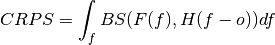
Continuous Ranked Probability Score (CRPS).
The CRPS can also be considered as the probabilistic Mean Absolute Error (
mae). It compares the empirical distribution of an ensemble forecast to a scalar observation. Smaller scores indicate better skill.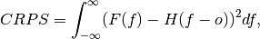
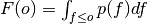
where
 is the cumulative distribution function (CDF) of the forecast
(since the verification data are not assigned a probability), and H() is the
Heaviside step function where the value is 1 if the argument is positive (i.e., the
forecast overestimates verification data) or zero (i.e., the forecast equals
verification data) and is 0 otherwise (i.e., the forecast is less than verification
data).
is the cumulative distribution function (CDF) of the forecast
(since the verification data are not assigned a probability), and H() is the
Heaviside step function where the value is 1 if the argument is positive (i.e., the
forecast overestimates verification data) or zero (i.e., the forecast equals
verification data) and is 0 otherwise (i.e., the forecast is less than verification
data).Note
The CRPS is expressed in the same unit as the observed variable. It generalizes the Mean Absolute Error (MAE), and reduces to the MAE if the forecast is determinstic.
- Parameters
forecast – Forecast with
memberdim.verif – Verification data without
memberdim.dim – Dimension to apply metric over. Expects at least
member. Other dimensions are passed toxskillscoreand averaged.metric_kwargs – optional, see
xskillscore.crps_ensemble()
Notes
minimum
0.0
maximum
∞
perfect
0.0
orientation
negative
References
Matheson and Winkler [1976]
See also
Example
>>> HindcastEnsemble.verify(
...     metric="crps", comparison="m2o", dim="member", alignment="same_inits"
... )
<xarray.Dataset>
Dimensions:     (lead: 10, init: 52)
Coordinates:
  * init        (init) object 1954-01-01 00:00:00 ... 2005-01-01 00:00:00
  * lead        (lead) int32 1 2 3 4 5 6 7 8 9 10
    valid_time  (lead, init) object 1955-01-01 00:00:00 ... 2015-01-01 00:00:00
    skill       <U11 'initialized'
Data variables:
    SST         (lead, init) float64 0.1722 0.1202 0.01764 ... 0.05428 0.1638
Attributes:
    prediction_skill_software:     climpred https://climpred.readthedocs.io/
    skill_calculated_by_function:  HindcastEnsemble.verify()
    number_of_members:             10
    alignment:                     same_inits
    metric:                        crps
    comparison:                    m2o
    dim:                           member
    reference:                     []
Continuous Ranked Probability Skill Score (CRPSS)
# Enter any of the below keywords in ``metric=...`` for the compute functions.
In [27]: print(f"Keywords: {metric_aliases['crpss']}")
Keywords: ['crpss']
- climpred.metrics._crpss(forecast: xarray.Dataset, verif: xarray.Dataset, dim: Optional[Union[str, List[str]]] = None, **metric_kwargs: Any) xarray.Dataset[source]
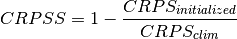
Continuous Ranked Probability Skill Score.
This can be used to assess whether the ensemble spread is a useful measure for the forecast uncertainty by comparing the CRPS of the ensemble forecast to that of a reference forecast with the desired spread.
Note
When assuming a Gaussian distribution of forecasts, use default
gaussian=True. If not gaussian, you may specify the distribution type,xmin/xmax/tolerancefor integration (seexskillscore.crps_quadrature()).- Parameters
forecast – Forecast with
memberdim.verif – Verification data without
memberdim.dim – Dimension to apply metric over. Expects at least
member. Other dimensions are passed toxskillscoreand averaged.gaussian (bool, optional) – If
True, assume Gaussian distribution for baseline skill. Defaults toTrue. seexskillscore.crps_ensemble(),xskillscore.crps_gaussian()andxskillscore.crps_quadrature()
Notes
minimum
-∞
maximum
1.0
perfect
1.0
orientation
positive
better than climatology
> 0.0
worse than climatology
< 0.0
References
Example
>>> HindcastEnsemble.verify(
...     metric="crpss", comparison="m2o", alignment="same_inits", dim="member"
... )
<xarray.Dataset>
Dimensions:     (init: 52, lead: 10)
Coordinates:
  * init        (init) object 1954-01-01 00:00:00 ... 2005-01-01 00:00:00
  * lead        (lead) int32 1 2 3 4 5 6 7 8 9 10
    valid_time  (lead, init) object 1955-01-01 00:00:00 ... 2015-01-01 00:00:00
    skill       <U11 'initialized'
Data variables:
    SST         (lead, init) float64 0.2644 0.3636 0.7376 ... 0.7702 0.5126
Attributes:
    prediction_skill_software:     climpred https://climpred.readthedocs.io/
    skill_calculated_by_function:  HindcastEnsemble.verify()
    number_of_members:             10
    alignment:                     same_inits
    metric:                        crpss
    comparison:                    m2o
    dim:                           member
    reference:                     []
>>> import scipy
>>> PerfectModelEnsemble.isel(lead=[0, 1]).verify(
...     metric="crpss",
...     comparison="m2m",
...     dim="member",
...     gaussian=False,
...     cdf_or_dist=scipy.stats.norm,
...     xmin=-10,
...     xmax=10,
...     tol=1e-6,
... )
<xarray.Dataset>
Dimensions:  (init: 12, lead: 2, member: 9)
Coordinates:
  * init     (init) object 3014-01-01 00:00:00 ... 3257-01-01 00:00:00
  * lead     (lead) int64 1 2
  * member   (member) int64 1 2 3 4 5 6 7 8 9
Data variables:
    tos      (lead, init, member) float64 0.9931 0.9932 0.9932 ... 0.9947 0.9947
See also
Continuous Ranked Probability Skill Score Ensemble Spread
# Enter any of the below keywords in ``metric=...`` for the compute functions.
In [28]: print(f"Keywords: {metric_aliases['crpss_es']}")
Keywords: ['crpss_es']
- climpred.metrics._crpss_es(forecast: xarray.Dataset, verif: xarray.Dataset, dim: Optional[Union[str, List[str]]] = None, **metric_kwargs: Any) xarray.Dataset[source]
Continuous Ranked Probability Skill Score Ensemble Spread.
If the ensemble variance is smaller than the observed
mse, the ensemble is said to be under-dispersive (or overconfident). An ensemble with variance larger than the verification data indicates one that is over-dispersive (underconfident).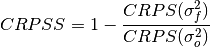
- Parameters
forecast – Forecast with
memberdim.verif – Verification data without
memberdim.dim – Dimension to apply metric over. Expects at least
member. Other dimensions are passed toxskillscoreand averaged.metric_kwargs – see
xskillscore.crps_ensemble()andxskillscore.mse()
Notes
minimum
-∞
maximum
0.0
perfect
0.0
orientation
positive
under-dispersive
> 0.0
over-dispersive
< 0.0
References
Kadow et al. [2016]
Example
>>> HindcastEnsemble.verify(
...     metric="crpss_es",
...     comparison="m2o",
...     alignment="same_verifs",
...     dim="member",
... )
<xarray.Dataset>
Dimensions:     (init: 52, lead: 10)
Coordinates:
  * init        (init) object 1964-01-01 00:00:00 ... 2015-01-01 00:00:00
  * lead        (lead) int32 1 2 3 4 5 6 7 8 9 10
    valid_time  (init) object 1964-01-01 00:00:00 ... 2015-01-01 00:00:00
    skill       <U11 'initialized'
Data variables:
    SST         (lead, init) float64 -0.01121 -0.05575 ... -0.1263 -0.007483
Attributes:
    prediction_skill_software:     climpred https://climpred.readthedocs.io/
    skill_calculated_by_function:  HindcastEnsemble.verify()
    number_of_members:             10
    alignment:                     same_verifs
    metric:                        crpss_es
    comparison:                    m2o
    dim:                           member
    reference:                     []
Brier Score
# Enter any of the below keywords in ``metric=...`` for the compute functions.
In [29]: print(f"Keywords: {metric_aliases['brier_score']}")
Keywords: ['brier_score', 'brier', 'bs']
- climpred.metrics._brier_score(forecast: xarray.Dataset, verif: xarray.Dataset, dim: Optional[Union[str, List[str]]] = None, **metric_kwargs: Any) xarray.Dataset[source]
Brier Score for binary events.
The Mean Square Error (
mse) of probabilistic two-category forecasts where the verification data are either 0 (no occurrence) or 1 (occurrence) and forecast probability may be arbitrarily distributed between occurrence and non-occurrence. The Brier Score equals zero for perfect (single-valued) forecasts and one for forecasts that are always incorrect.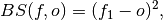
where
 is the forecast probability of
  .
.Note
The Brier Score requires that the observation is binary, i.e., can be described as one (a “hit”) or zero (a “miss”). So either provide a function with with binary outcomes
logicalinmetric_kwargsor create binary verifs and probability forecasts by hindcast.map(logical).mean(“member”). This Brier Score is not the original formula given in Brier [1950].- Parameters
forecast – Raw forecasts with
memberdimension iflogicalprovided in metric_kwargs. Probability forecasts in[0, 1]iflogicalis not provided.verif – Verification data without
memberdim. Raw verification iflogicalprovided, else binary verification.dim – Dimensions to aggregate. Requires
memberiflogicalprovided inmetric_kwargs``to create probability forecasts. If ``logicalnot provided inmetric_kwargs, should not includemember.logical (callable) – Function with bool result to be applied to verification data and forecasts and then
mean("member")to get forecasts and verification data in interval[0, 1]. seexskillscore.brier_score()
Notes
minimum
0.0
maximum
1.0
perfect
0.0
orientation
negative
References
See also
Example
Define a boolean/logical: Function for binary scoring:
>>> def pos(x):
...     return x > 0  # checking binary outcomes
...
Option 1. Pass with keyword
logical: (specifically designed forPerfectModelEnsemble, where binary verification can only be created after comparison)>>> HindcastEnsemble.verify( ... metric="brier_score", ... comparison="m2o", ... dim=["member", "init"], ... alignment="same_verifs", ... logical=pos, ... ) <xarray.Dataset> Dimensions: (lead: 10) Coordinates: * lead (lead) int32 1 2 3 4 5 6 7 8 9 10 skill <U11 'initialized' Data variables: SST (lead) float64 0.115 0.1121 0.1363 0.125 ... 0.1654 0.1675 0.1873 Attributes: prediction_skill_software: climpred https://climpred.readthedocs.io/ skill_calculated_by_function: HindcastEnsemble.verify() number_of_initializations: 64 number_of_members: 10 alignment: same_verifs metric: brier_score comparison: m2o dim: ['member', 'init'] reference: [] logical: Callable
Option 2. Pre-process to generate a binary multi-member forecast and binary verification product:
>>> HindcastEnsemble.map(pos).verify(
...     metric="brier_score",
...     comparison="m2o",
...     dim=["member", "init"],
...     alignment="same_verifs",
... )
<xarray.Dataset>
Dimensions:  (lead: 10)
Coordinates:
  * lead     (lead) int32 1 2 3 4 5 6 7 8 9 10
    skill    <U11 'initialized'
Data variables:
    SST      (lead) float64 0.115 0.1121 0.1363 0.125 ... 0.1654 0.1675 0.1873
Attributes:
    prediction_skill_software:     climpred https://climpred.readthedocs.io/
    skill_calculated_by_function:  HindcastEnsemble.verify()
    number_of_initializations:     64
    number_of_members:             10
    alignment:                     same_verifs
    metric:                        brier_score
    comparison:                    m2o
    dim:                           ['member', 'init']
    reference:                     []
Option 3. Pre-process to generate a probability forecast and binary verification product. because
membernot present inhindcastanymore, usecomparison="e2o"anddim="init":>>> HindcastEnsemble.map(pos).mean("member").verify( ... metric="brier_score", ... comparison="e2o", ... dim="init", ... alignment="same_verifs", ... ) <xarray.Dataset> Dimensions: (lead: 10) Coordinates: * lead (lead) int32 1 2 3 4 5 6 7 8 9 10 skill <U11 'initialized' Data variables: SST (lead) float64 0.115 0.1121 0.1363 0.125 ... 0.1654 0.1675 0.1873 Attributes: prediction_skill_software: climpred https://climpred.readthedocs.io/ skill_calculated_by_function: HindcastEnsemble.verify() number_of_initializations: 64 alignment: same_verifs metric: brier_score comparison: e2o dim: init reference: []
Threshold Brier Score
# Enter any of the below keywords in ``metric=...`` for the compute functions.
In [30]: print(f"Keywords: {metric_aliases['threshold_brier_score']}")
Keywords: ['threshold_brier_score', 'tbs']
- climpred.metrics._threshold_brier_score(forecast: xarray.Dataset, verif: xarray.Dataset, dim: Optional[Union[str, List[str]]] = None, **metric_kwargs: Any) xarray.Dataset[source]
Brier score of an ensemble for exceeding given thresholds.
where
 is the cumulative distribution
function (CDF) of the forecast distribution
is the cumulative distribution
function (CDF) of the forecast distribution  ,
,  is a point estimate
of the true observation (observational error is neglected),
is a point estimate
of the true observation (observational error is neglected),  denotes the
Brier score and
denotes the
Brier score and  denotes the Heaviside step function, which we define
here as equal to 1 for
denotes the Heaviside step function, which we define
here as equal to 1 for  and 0 otherwise.
- Parameters
forecast – Forecast with
memberdim.verif – Verification data without
memberdim.dim – Dimension to apply metric over. Expects at least
member. Other dimensions are passed toxskillscoreand averaged.threshold (int, float, xarray.Dataset, xr.DataArray) – Threshold to check exceedance, see
xskillscore.threshold_brier_score().metric_kwargs – optional, see
xskillscore.threshold_brier_score()
Notes
minimum
0.0
maximum
1.0
perfect
0.0
orientation
negative
References
Brier [1950]
See also
Example
>>> # get threshold brier score for each init
>>> HindcastEnsemble.verify(
...     metric="threshold_brier_score",
...     comparison="m2o",
...     dim="member",
...     threshold=0.2,
...     alignment="same_inits",
... )
<xarray.Dataset>
Dimensions:     (lead: 10, init: 52)
Coordinates:
  * init        (init) object 1954-01-01 00:00:00 ... 2005-01-01 00:00:00
  * lead        (lead) int32 1 2 3 4 5 6 7 8 9 10
    valid_time  (lead, init) object 1955-01-01 00:00:00 ... 2015-01-01 00:00:00
    threshold   float64 0.2
    skill       <U11 'initialized'
Data variables:
    SST         (lead, init) float64 0.0 0.0 0.0 0.0 0.0 ... 0.25 0.36 0.09 0.01
Attributes:
    prediction_skill_software:     climpred https://climpred.readthedocs.io/
    skill_calculated_by_function:  HindcastEnsemble.verify()
    number_of_members:             10
    alignment:                     same_inits
    metric:                        threshold_brier_score
    comparison:                    m2o
    dim:                           member
    reference:                     []
    threshold:                     0.2
>>> # multiple thresholds averaging over init dimension
>>> HindcastEnsemble.verify(
...     metric="threshold_brier_score",
...     comparison="m2o",
...     dim=["member", "init"],
...     threshold=[0.2, 0.3],
...     alignment="same_verifs",
... )
<xarray.Dataset>
Dimensions:    (lead: 10, threshold: 2)
Coordinates:
  * lead       (lead) int32 1 2 3 4 5 6 7 8 9 10
  * threshold  (threshold) float64 0.2 0.3
    skill      <U11 'initialized'
Data variables:
    SST        (lead, threshold) float64 0.08712 0.005769 ... 0.1312 0.01923
Attributes:
    prediction_skill_software:     climpred https://climpred.readthedocs.io/
    skill_calculated_by_function:  HindcastEnsemble.verify()
    number_of_initializations:     64
    number_of_members:             10
    alignment:                     same_verifs
    metric:                        threshold_brier_score
    comparison:                    m2o
    dim:                           ['member', 'init']
    reference:                     []
    threshold:                     [0.2, 0.3]
Ranked Probability Score
# Enter any of the below keywords in ``metric=...`` for the compute functions.
In [31]: print(f"Keywords: {metric_aliases['rps']}")
Keywords: ['rps']
- climpred.metrics._rps(forecast: xarray.Dataset, verif: xarray.Dataset, dim: Optional[Union[str, List[str]]] = None, **metric_kwargs: Any) xarray.Dataset[source]
Ranked Probability Score.
![RPS(p, k) = \sum_{m=1}^{M} [(\sum_{k=1}^{m} p_k) - (\sum_{k=1}^{m} \
o_k)]^{2}](_images/math/cc31dcad7fe9027635df9bc074a0f5f52a8fa936.png)
- Parameters
forecast – Forecasts.
verif – Verification.
dim – Dimensions to aggregate.
**metric_kwargs, see :py:func:`.xskillscore.rps`
Note
If
category_edgesis xr.Dataset or tuple of xr.Datasets, climpred will broadcast the grouped dimensionsseason,month,weekofyear,dayfofyearonto the dimensionsinitfor forecast andtimefor observations. seeclimpred.utils.broadcast_time_grouped_to_time.Notes
minimum
0.0
maximum
∞
perfect
0.0
orientation
negative
See also
Example
>>> category_edges = np.array([-0.5, 0.0, 0.5, 1.0])
>>> HindcastEnsemble.verify(
...     metric="rps",
...     comparison="m2o",
...     dim=["member", "init"],
...     alignment="same_verifs",
...     category_edges=category_edges,
... )
<xarray.Dataset>
Dimensions:                     (lead: 10)
Coordinates:
  * lead                        (lead) int32 1 2 3 4 5 6 7 8 9 10
    observations_category_edge  <U67 '[-np.inf, -0.5), [-0.5, 0.0), [0.0, 0.5...
    forecasts_category_edge     <U67 '[-np.inf, -0.5), [-0.5, 0.0), [0.0, 0.5...
    skill                       <U11 'initialized'
Data variables:
    SST                         (lead) float64 0.115 0.1123 ... 0.1687 0.1875
Attributes:
    prediction_skill_software:     climpred https://climpred.readthedocs.io/
    skill_calculated_by_function:  HindcastEnsemble.verify()
    number_of_initializations:     64
    number_of_members:             10
    alignment:                     same_verifs
    metric:                        rps
    comparison:                    m2o
    dim:                           ['member', 'init']
    reference:                     []
    category_edges:                [-0.5  0.   0.5  1. ]
Provide
category_edgesasxarray.Datasetfor category edges varying along dimensions.>>> category_edges = ( ... xr.DataArray([9.5, 10.0, 10.5, 11.0], dims="category_edge") ... .assign_coords(category_edge=[9.5, 10.0, 10.5, 11.0]) ... .to_dataset(name="tos") ... ) >>> # category_edges = np.array([9.5, 10., 10.5, 11.]) # identical >>> PerfectModelEnsemble.verify( ... metric="rps", ... comparison="m2c", ... dim=["member", "init"], ... category_edges=category_edges, ... ) <xarray.Dataset> Dimensions: (lead: 20) Coordinates: * lead (lead) int64 1 2 3 4 5 6 7 ... 15 16 17 18 19 20 observations_category_edge <U71 '[-np.inf, 9.5), [9.5, 10.0), [10.0, 10.... forecasts_category_edge <U71 '[-np.inf, 9.5), [9.5, 10.0), [10.0, 10.... Data variables: tos (lead) float64 0.08951 0.1615 ... 0.1399 0.2274 Attributes: prediction_skill_software: climpred https://climpred.readthedocs.io/ skill_calculated_by_function: PerfectModelEnsemble.verify() number_of_initializations: 12 number_of_members: 10 metric: rps comparison: m2c dim: ['member', 'init'] reference: [] category_edges: <xarray.Dataset>\nDimensions: (cate...
Provide
category_edgesas tuple for different category edges to categorize forecasts and observations.>>> q = [1 / 3, 2 / 3] # terciles by month >>> forecast_edges = ( ... HindcastEnsemble.get_initialized() ... .groupby("init.month") ... .quantile(q=q, dim=["init", "member"]) ... .rename({"quantile": "category_edge"}) ... ) >>> obs_edges = ( ... HindcastEnsemble.get_observations() ... .groupby("time.month") ... .quantile(q=q, dim="time") ... .rename({"quantile": "category_edge"}) ... ) >>> category_edges = (obs_edges, forecast_edges) >>> HindcastEnsemble.verify( ... metric="rps", ... comparison="m2o", ... dim=["member", "init"], ... alignment="same_verifs", ... category_edges=category_edges, ... ) <xarray.Dataset> Dimensions: (lead: 10) Coordinates: * lead (lead) int32 1 2 3 4 5 6 7 8 9 10 observations_category_edge <U101 '[-np.inf, 0.3333333333333333), [0.3333... forecasts_category_edge <U101 '[-np.inf, 0.3333333333333333), [0.3333... skill <U11 'initialized' Data variables: SST (lead) float64 0.1248 0.1756 ... 0.3081 0.3413 Attributes: prediction_skill_software: climpred https://climpred.readthedocs.io/ skill_calculated_by_function: HindcastEnsemble.verify() number_of_initializations: 64 number_of_members: 10 alignment: same_verifs metric: rps comparison: m2o dim: ['member', 'init'] reference: [] category_edges: (<xarray.Dataset>\nDimensions: (mon...
Reliability
# Enter any of the below keywords in ``metric=...`` for the compute functions.
In [32]: print(f"Keywords: {metric_aliases['reliability']}")
Keywords: ['reliability']
- climpred.metrics._reliability(forecast: xarray.Dataset, verif: xarray.Dataset, dim: Optional[Union[str, List[str]]] = None, **metric_kwargs: Any) xarray.Dataset[source]
Reliability.
Returns the data required to construct the reliability diagram for an event. The the relative frequencies of occurrence of an event for a range of forecast probability bins.
- Parameters
forecast – Raw forecasts with
memberdimension iflogicalprovided inmetric_kwargs. Probability forecasts in[0, 1]iflogicalis not provided.verif – Verification data without
memberdim. Raw verification iflogicalprovided, else binary verification.dim – Dimensions to aggregate. Requires
memberiflogicalprovided inmetric_kwargs``to create probability forecasts. If ``logicalnot provided inmetric_kwargs, should not includemember.logical – Function with bool result to be applied to verification data and forecasts and then
mean("member")to get forecasts and verification data in interval[0, 1]. Passed viametric_kwargs.probability_bin_edges (array_like, optional) – Probability bin edges used to compute the reliability. Bins include the left most edge, but not the right. Passed via
metric_kwargs. Defaults to 6 equally spaced edges between0and1+1e-8.
- Returns
reliability – The relative frequency of occurrence for each probability bin
Notes
perfect
flat distribution
See also
Example
Define a boolean/logical: Function for binary scoring:
>>> def pos(x):
...     return x > 0  # checking binary outcomes
...
Option 1. Pass with keyword
logical: (especially designed forPerfectModelEnsemble, where binary verification can only be created after comparison))>>> HindcastEnsemble.verify( ... metric="reliability", ... comparison="m2o", ... dim=["member", "init"], ... alignment="same_verifs", ... logical=pos, ... ) <xarray.Dataset> Dimensions: (lead: 10, forecast_probability: 5) Coordinates: * lead (lead) int32 1 2 3 4 5 6 7 8 9 10 * forecast_probability (forecast_probability) float64 0.1 0.3 0.5 0.7 0.9 SST_samples (lead, forecast_probability) float64 22.0 5.0 ... 13.0 skill <U11 'initialized' Data variables: SST (lead, forecast_probability) float64 0.09091 ... 1.0 Attributes: prediction_skill_software: climpred https://climpred.readthedocs.io/ skill_calculated_by_function: HindcastEnsemble.verify() number_of_initializations: 64 number_of_members: 10 alignment: same_verifs metric: reliability comparison: m2o dim: ['member', 'init'] reference: [] logical: Callable
Option 2. Pre-process to generate a binary forecast and verification product:
>>> HindcastEnsemble.map(pos).verify(
...     metric="reliability",
...     comparison="m2o",
...     dim=["init", "member"],
...     alignment="same_verifs",
... )
<xarray.Dataset>
Dimensions:               (lead: 10, forecast_probability: 5)
Coordinates:
  * lead                  (lead) int32 1 2 3 4 5 6 7 8 9 10
  * forecast_probability  (forecast_probability) float64 0.1 0.3 0.5 0.7 0.9
    SST_samples           (lead, forecast_probability) float64 22.0 5.0 ... 13.0
    skill                 <U11 'initialized'
Data variables:
    SST                   (lead, forecast_probability) float64 0.09091 ... 1.0
Attributes:
    prediction_skill_software:     climpred https://climpred.readthedocs.io/
    skill_calculated_by_function:  HindcastEnsemble.verify()
    number_of_initializations:     64
    number_of_members:             10
    alignment:                     same_verifs
    metric:                        reliability
    comparison:                    m2o
    dim:                           ['init', 'member']
    reference:                     []
Option 3. Pre-process to generate a probability forecast and binary verification product. because
membernot present inhindcast, usecomparison="e2o"anddim="init":>>> HindcastEnsemble.map(pos).mean("member").verify( ... metric="reliability", ... comparison="e2o", ... dim="init", ... alignment="same_verifs", ... ) <xarray.Dataset> Dimensions: (lead: 10, forecast_probability: 5) Coordinates: * lead (lead) int32 1 2 3 4 5 6 7 8 9 10 * forecast_probability (forecast_probability) float64 0.1 0.3 0.5 0.7 0.9 SST_samples (lead, forecast_probability) float64 22.0 5.0 ... 13.0 skill <U11 'initialized' Data variables: SST (lead, forecast_probability) float64 0.09091 ... 1.0 Attributes: prediction_skill_software: climpred https://climpred.readthedocs.io/ skill_calculated_by_function: HindcastEnsemble.verify() number_of_initializations: 64 alignment: same_verifs metric: reliability comparison: e2o dim: init reference: []
Discrimination
# Enter any of the below keywords in ``metric=...`` for the compute functions.
In [33]: print(f"Keywords: {metric_aliases['discrimination']}")
Keywords: ['discrimination']
- climpred.metrics._discrimination(forecast: xarray.Dataset, verif: xarray.Dataset, dim: Optional[Union[str, List[str]]] = None, **metric_kwargs: Any) xarray.Dataset[source]
Discrimination.
Return the data required to construct the discrimination diagram for an event. The histogram of forecasts likelihood when observations indicate an event has occurred and has not occurred.
- Parameters
forecast – Raw forecasts with
memberdimension iflogicalprovided in metric_kwargs. Probability forecasts in [0, 1] iflogicalis not provided.verif – Verification data without
memberdim. Raw verification iflogicalprovided, else binary verification.dim – Dimensions to aggregate. Requires
memberiflogicalprovided inmetric_kwargsto create probability forecasts. Iflogicalnot provided inmetric_kwargs, should not includemember. At least one dimension other than ``member``is required.logical – Function with bool result to be applied to verification data and forecasts and then
mean("member")to get forecasts and verification data in interval[0, 1]. Passed viametric_kwargs.probability_bin_edges (array_like, optional) – Probability bin edges used to compute the histograms. Bins include the left most edge, but not the right. Passed via
metric_kwargs. Defaults to 6 equally spaced edges between0and1+1e-8.
- Returns
Discrimination with added dimension
eventcontaining the histograms of forecast probabilities when the event was observed and not observed.
Notes
perfect
distinct distributions
See also
Example
Define a boolean/logical: Function for binary scoring:
>>> def pos(x):
...     return x > 0  # checking binary outcomes
...
Option 1. Pass with keyword
logical: (especially designed forPerfectModelEnsemble, where binary verification can only be created after comparison)>>> HindcastEnsemble.verify( ... metric="discrimination", ... comparison="m2o", ... dim=["member", "init"], ... alignment="same_verifs", ... logical=pos, ... ) <xarray.Dataset> Dimensions: (lead: 10, forecast_probability: 5, event: 2) Coordinates: * lead (lead) int32 1 2 3 4 5 6 7 8 9 10 * forecast_probability (forecast_probability) float64 0.1 0.3 0.5 0.7 0.9 * event (event) bool True False skill <U11 'initialized' Data variables: SST (lead, event, forecast_probability) float64 0.07407...
Option 2. Pre-process to generate a binary forecast and verification product:
>>> HindcastEnsemble.map(pos).verify(
...     metric="discrimination",
...     comparison="m2o",
...     dim=["member", "init"],
...     alignment="same_verifs",
... )
<xarray.Dataset>
Dimensions:               (lead: 10, forecast_probability: 5, event: 2)
Coordinates:
  * lead                  (lead) int32 1 2 3 4 5 6 7 8 9 10
  * forecast_probability  (forecast_probability) float64 0.1 0.3 0.5 0.7 0.9
  * event                 (event) bool True False
    skill                 <U11 'initialized'
Data variables:
    SST                   (lead, event, forecast_probability) float64 0.07407...
Option 3. Pre-process to generate a probability forecast and binary verification product. because
membernot present inhindcast, usecomparison="e2o"anddim="init":>>> HindcastEnsemble.map(pos).mean("member").verify( ... metric="discrimination", ... comparison="e2o", ... dim="init", ... alignment="same_verifs", ... ) <xarray.Dataset> Dimensions: (lead: 10, forecast_probability: 5, event: 2) Coordinates: * lead (lead) int32 1 2 3 4 5 6 7 8 9 10 * forecast_probability (forecast_probability) float64 0.1 0.3 0.5 0.7 0.9 * event (event) bool True False skill <U11 'initialized' Data variables: SST (lead, event, forecast_probability) float64 0.07407...
Rank Histogram
# Enter any of the below keywords in ``metric=...`` for the compute functions.
In [34]: print(f"Keywords: {metric_aliases['rank_histogram']}")
Keywords: ['rank_histogram']
- climpred.metrics._rank_histogram(forecast: xarray.Dataset, verif: xarray.Dataset, dim: Optional[Union[str, List[str]]] = None, **metric_kwargs: Any) xarray.Dataset[source]
Rank histogram or Talagrand diagram.
- Parameters
forecast – Raw forecasts with
memberdimension.verif – Verification data without
memberdim.dim – Dimensions to aggregate. Requires to contain
memberand at least one additional dimension.
Notes
flat
perfect
slope
biased
u-shaped
overconfident/underdisperive
dome-shaped
underconfident/overdisperive
See also
Example
>>> HindcastEnsemble.verify(
...     metric="rank_histogram",
...     comparison="m2o",
...     dim=["member", "init"],
...     alignment="same_verifs",
... )
<xarray.Dataset>
Dimensions:  (lead: 10, rank: 11)
Coordinates:
  * lead     (lead) int32 1 2 3 4 5 6 7 8 9 10
  * rank     (rank) float64 1.0 2.0 3.0 4.0 5.0 6.0 7.0 8.0 9.0 10.0 11.0
    skill    <U11 'initialized'
Data variables:
    SST      (lead, rank) int64 12 3 2 1 1 3 1 2 6 5 16 ... 0 1 0 0 3 0 2 6 6 34
Attributes:
    prediction_skill_software:     climpred https://climpred.readthedocs.io/
    skill_calculated_by_function:  HindcastEnsemble.verify()
    number_of_initializations:     64
    number_of_members:             10
    alignment:                     same_verifs
    metric:                        rank_histogram
    comparison:                    m2o
    dim:                           ['member', 'init']
    reference:                     []
>>> PerfectModelEnsemble.verify(
...     metric="rank_histogram", comparison="m2c", dim=["member", "init"]
... )
<xarray.Dataset>
Dimensions:  (lead: 20, rank: 10)
Coordinates:
  * lead     (lead) int64 1 2 3 4 5 6 7 8 9 10 11 12 13 14 15 16 17 18 19 20
  * rank     (rank) float64 1.0 2.0 3.0 4.0 5.0 6.0 7.0 8.0 9.0 10.0
Data variables:
    tos      (lead, rank) int64 1 4 2 1 2 1 0 0 0 1 2 ... 0 2 0 1 2 1 0 3 1 2 0
Attributes:
    prediction_skill_software:     climpred https://climpred.readthedocs.io/
    skill_calculated_by_function:  PerfectModelEnsemble.verify()
    number_of_initializations:     12
    number_of_members:             10
    metric:                        rank_histogram
    comparison:                    m2c
    dim:                           ['member', 'init']
    reference:                     []
Logarithmic Ensemble Spread Score
# Enter any of the below keywords in ``metric=...`` for the compute functions.
In [35]: print(f"Keywords: {metric_aliases['less']}")
Keywords: ['less']
- climpred.metrics._less(forecast: xarray.Dataset, verif: xarray.Dataset, dim: Optional[Union[str, List[str]]] = None, **metric_kwargs: Any) xarray.Dataset[source]
Logarithmic Ensemble Spread Score.
- Parameters
forecast – Forecasts.
verif – Verification.
dim – The dimension(s) over which to aggregate. Defaults to None, meaning aggregation over all dims other than
lead.
- Returns
less – reduced by dimensions
dim
Notes
maximum
∞
positive
overdisperive / underconfident
perfect
0
negative
underdisperive / overconfident
minimum
-∞
orientation
None
Example
>>> # better detrend before
>>> from climpred.stats import rm_poly
>>> HindcastEnsemble.map(rm_poly, dim="init_or_time", deg=2).verify(
...     metric="less",
...     comparison="m2o",
...     dim=["member", "init"],
...     alignment="same_verifs",
... ).SST
<xarray.DataArray 'SST' (lead: 10)>
array([ 0.12633664, -0.12707636, -0.26143181, -0.25096537, -0.29267366,
       -0.2905725 , -0.43579508, -0.33774947, -0.46008438, -0.61010386])
Coordinates:
  * lead     (lead) int32 1 2 3 4 5 6 7 8 9 10
    skill    <U11 'initialized'
Attributes:
    units:    None
References
Kadow et al. [2016]
Contingency-based metrics
Contingency
A number of metrics can be derived from a contingency table. To use this in climpred, run .verify(metric='contingency', score=...) where score can be chosen from xskillscore.
- climpred.metrics._contingency(forecast, verif, score='table', dim=None, **metric_kwargs)[source]
Contingency table.
- Parameters
forecast – Raw forecasts.
verif – Verification data.
dim – Dimensions to aggregate.
score (str) – Score derived from contingency table. Attribute from
Contingency. Usescore=tableto return a contingency table or any other contingency score, e.g.score=hit_rate.observation_category_edges (array_like) – Category bin edges used to compute the observations CDFs. Bins include the left most edge, but not the right. Passed via
metric_kwargs.forecast_category_edges (array_like) – Category bin edges used to compute the forecast CDFs. Bins include the left most edge, but not the right. Passed via metric_kwargs
See also
Example
>>> category_edges = np.array([-0.5, 0.0, 0.5, 1.0])
>>> HindcastEnsemble.verify(
...     metric="contingency",
...     score="table",
...     comparison="m2o",
...     dim=["member", "init"],
...     alignment="same_verifs",
...     observation_category_edges=category_edges,
...     forecast_category_edges=category_edges,
... ).isel(lead=[0, 1]).SST
<xarray.DataArray 'SST' (lead: 2, observations_category: 3, forecasts_category: 3)>
array([[[221,  29,   0],
        [ 53, 217,   0],
        [  0,   0,   0]],

       [[234,  16,   0],
        [ 75, 194,   1],
        [  0,   0,   0]]])
Coordinates:
  * lead                          (lead) int32 1 2
    observations_category_bounds  (observations_category) <U11 '[-0.5, 0.0)' ...
    forecasts_category_bounds     (forecasts_category) <U11 '[-0.5, 0.0)' ......
  * observations_category         (observations_category) int64 1 2 3
  * forecasts_category            (forecasts_category) int64 1 2 3
    skill                         <U11 'initialized'
Attributes:
    units:    None
>>> # contingency-based dichotomous accuracy score
>>> category_edges = np.array([9.5, 10.0, 10.5])
>>> PerfectModelEnsemble.verify(
...     metric="contingency",
...     score="hit_rate",
...     comparison="m2c",
...     dim=["member", "init"],
...     observation_category_edges=category_edges,
...     forecast_category_edges=category_edges,
... )
<xarray.Dataset>
Dimensions:  (lead: 20)
Coordinates:
  * lead     (lead) int64 1 2 3 4 5 6 7 8 9 10 11 12 13 14 15 16 17 18 19 20
Data variables:
    tos      (lead) float64 1.0 1.0 1.0 1.0 0.9091 ... 1.0 1.0 1.0 nan 1.0
Attributes:
    prediction_skill_software:     climpred https://climpred.readthedocs.io/
    skill_calculated_by_function:  PerfectModelEnsemble.verify()
    number_of_initializations:     12
    number_of_members:             10
    metric:                        contingency
    comparison:                    m2c
    dim:                           ['member', 'init']
    reference:                     []
    score:                         hit_rate
    observation_category_edges:    [ 9.5 10.  10.5]
    forecast_category_edges:       [ 9.5 10.  10.5]
Receiver Operating Characteristic
# Enter any of the below keywords in ``metric=...`` for the compute functions.
In [36]: print(f"Keywords: {metric_aliases['roc']}")
Keywords: ['roc', 'Receiver Operating Characteristic', 'receiver_operating_characteristic']
- climpred.metrics._roc(forecast: xarray.Dataset, verif: xarray.Dataset, dim: Optional[Union[str, List[str]]] = None, **metric_kwargs: Any) xarray.Dataset[source]
Receiver Operating Characteristic.
- Parameters
observations – Labeled array(s) over which to apply the function. If
bin_edges=="continuous", observations are binary.forecasts – Labeled array(s) over which to apply the function. If
bin_edges=="continuous", forecasts are probabilities.dim – The dimension(s) over which to aggregate. Defaults to None, meaning aggregation over all dims other than
lead.logical – Function with bool result to be applied to verification data and forecasts and then
mean("member")to get forecasts and verification data in interval[0, 1]. Passed viametric_kwargs.bin_edges (array_like, str) – Bin edges for categorising observations and forecasts. Similar to np.histogram, all but the last (righthand-most) bin include the left edge and exclude the right edge. The last bin includes both edges.
bin_edgeswill be sorted in ascending order. Ifbin_edges=="continuous", calculatebin_edgesfrom forecasts, equal tosklearn.metrics.roc_curve(f_boolean, o_prob). Passed viametric_kwargs. Defaults to “continuous”.drop_intermediate (bool) – Whether to drop some suboptimal thresholds which would not appear on a plotted ROC curve. This is useful in order to create lighter ROC curves. Defaults to
False. Defaults toTrueinsklearn.metrics.roc_curve. Passed viametric_kwargs.return_results (str) – Passed via
metric_kwargs. Defaults to “area”. Specify how return is structed:“area”: return only the
area under curveof ROC“all_as_tuple”: return
true positive rateandfalse positive rateat each bin and area under the curve of ROC as tuple“all_as_metric_dim”: return
true positive rateandfalse positive rateat each bin andarea under curveof ROC concatinated into newmetricdimension
- Returns
reduced by dimensions
dim, seereturn_resultsparameter.true positive rateandfalse positive ratecontainprobability_bindimension with ascendingbin_edgesas coordinates.
Notes
minimum
0.0
maximum
1.0
perfect
1.0
orientation
positive
See also
Example
>>> bin_edges = np.array([-0.5, 0.0, 0.5, 1.0])
>>> HindcastEnsemble.verify(
...     metric="roc",
...     comparison="m2o",
...     dim=["member", "init"],
...     alignment="same_verifs",
...     bin_edges=bin_edges,
... ).SST
<xarray.DataArray 'SST' (lead: 10)>
array([0.84385185, 0.82841667, 0.81358547, 0.8393463 , 0.82551752,
       0.81987778, 0.80719573, 0.80081909, 0.79046553, 0.78037564])
Coordinates:
  * lead     (lead) int32 1 2 3 4 5 6 7 8 9 10
    skill    <U11 'initialized'
Attributes:
    units:    None
Get area under the curve, false positive rate and true positive rate as
metricdimension by specifyingreturn_results="all_as_metric_dim":>>> def f(ds): ... return ds > 0 ... >>> HindcastEnsemble.map(f).verify( ... metric="roc", ... comparison="m2o", ... dim=["member", "init"], ... alignment="same_verifs", ... bin_edges="continuous", ... return_results="all_as_metric_dim", ... ).SST.isel(lead=[0, 1]) <xarray.DataArray 'SST' (lead: 2, metric: 3, probability_bin: 3)> array([[[0. , 0.116 , 1. ], [0. , 0.8037037 , 1. ], [0.84385185, 0.84385185, 0.84385185]], [[0. , 0.064 , 1. ], [0. , 0.72222222, 1. ], [0.82911111, 0.82911111, 0.82911111]]]) Coordinates: * probability_bin (probability_bin) float64 2.0 1.0 0.0 * lead (lead) int32 1 2 * metric (metric) <U19 'false positive rate' ... 'area under curve' skill <U11 'initialized' Attributes: units: None
User-defined metrics
You can also construct your own metrics via the climpred.metrics.Metric
class.
|
Master class for all metrics. |
First, write your own metric function, similar to the existing ones with required
arguments forecast, observations, dim=None, and **metric_kwargs:
from climpred.metrics import Metric

def _my_msle(forecast, observations, dim=None, **metric_kwargs):
    """Mean squared logarithmic error (MSLE).
    https://peltarion.com/knowledge-center/documentation/modeling-view/build-an-ai-model/loss-functions/mean-squared-logarithmic-error."""
    # function
    return ( (np.log(forecast + 1) + np.log(observations + 1) ) ** 2).mean(dim)
Then initialize this metric function with climpred.metrics.Metric:
_my_msle = Metric(
    name='my_msle',
    function=_my_msle,
    probabilistic=False,
    positive=False,
    unit_power=0,
    )
Finally, compute skill based on your own metric:
skill = hindcast.verify(metric=_my_msle, comparison='e2o', alignment='same_verif', dim='init')
Once you come up with an useful metric for your problem, consider contributing this metric to climpred, so all users can benefit from your metric, see contributing.
References
- 1(1,2,3)
Christopher S. Bretherton, Martin Widmann, Valentin P. Dymnikov, John M. Wallace, and Ileana Bladé. The Effective Number of Spatial Degrees of Freedom of a Time-Varying Field. Journal of Climate, 12(7):1990–2009, July 1999. doi:10/bs7fv4.
- 2(1,2,3)
Glenn W. Brier. Verficiation of forecasts expressed int terms of probability. Monthly Weather Review, 1950. doi:10.1175/1520-0493(1950)078<0001:VOFEIT>2.0.CO;2.
- 3(1,2,3,4)
Mitchell Bushuk, Rym Msadek, Michael Winton, Gabriel Vecchi, Xiaosong Yang, Anthony Rosati, and Rich Gudgel. Regional Arctic sea–ice prediction: potential versus operational seasonal forecast skill. Climate Dynamics, June 2018. doi:10/gd7hfq.
- 4
Tilmann Gneiting and Adrian E Raftery. Strictly Proper Scoring Rules, Prediction, and Estimation. Journal of the American Statistical Association, 102(477):359–378, March 2007. doi:10/c6758w.
- 5(1,2,3)
S. M. Griffies and K. Bryan. A predictability study of simulated North Atlantic multidecadal variability. Climate Dynamics, 13(7-8):459–487, August 1997. doi:10/ch4kc4.
- 6
Ed Hawkins, Buwen Dong, Jon Robson, Rowan Sutton, and Doug Smith. The Interpretation and Use of Biases in Decadal Climate Predictions. Journal of Climate, 27(8):2931–2947, January 2014. doi:10/f5w2xr.
- 7(1,2,3,4)
Ian T. Jolliffe and David B. Stephenson. Forecast Verification: A Practitioner's Guide in Atmospheric Science. John Wiley & Sons, Ltd, Chichester, UK, December 2011. ISBN 978-1-119-96000-3 978-0-470-66071-3. doi:10.1002/9781119960003.
- 8(1,2)
Christopher Kadow, Sebastian Illing, Oliver Kunst, Henning W. Rust, Holger Pohlmann, Wolfgang A. Müller, and Ulrich Cubasch. Evaluation of forecasts by accuracy and spread in the MiKlip decadal climate prediction system. Meteorologische Zeitschrift, pages 631–643, December 2016. doi:10/f9jrhw.
- 9(1,2)
James E. Matheson and Robert L. Winkler. Scoring Rules for Continuous Probability Distributions. Management Science, 22(10):1087–1096, June 1976. doi:10/cwwt4g.
- 10(1,2,3,4,5,6,7,8,9,10,11)
Allan H. Murphy. Skill Scores Based on the Mean Square Error and Their Relationships to the Correlation Coefficient. Monthly Weather Review, 116(12):2417–2424, December 1988. doi:10/fc7mxd.
- 11
Holger Pohlmann, Michael Botzet, Mojib Latif, Andreas Roesch, Martin Wild, and Peter Tschuck. Estimating the Decadal Predictability of a Coupled AOGCM. Journal of Climate, 17(22):4463–4472, November 2004. doi:10/d2qf62.