You can run this notebook in a live session ![]() or view it on Github.
or view it on Github.
Calculate Seasonal ENSO Skill of the NMME model NCEP-CFSv2
In this example, we demonstrate:
How to remotely access data from the North American Multi-model Ensemble (NMME) hindcast database and set it up to be used in
climpredHow to calculate the Anomaly Correlation Coefficient (ACC) using seasonal data
The North American Multi-model Ensemble (NMME)
Further information on NMME is available from Kirtman et al. [2014] and the NMME project website.
The NMME public database is hosted on the International Research Institute for Climate and Society (IRI) data server http://iridl.ldeo.columbia.edu/SOURCES/.Models/.NMME/.
Definitions
- Anomalies
Departure from normal, where normal is defined as the climatological value based on the average value for each month over all years.
- Nino3.4
An index used to represent the evolution of the El Nino-Southern Oscillation (ENSO). Calculated as the average sea surface temperature (SST) anomalies in the region 5S-5N; 190-240
# linting
%load_ext nb_black
%load_ext lab_black
import matplotlib.pyplot as plt
import xarray as xr
import pandas as pd
import numpy as np

from climpred import HindcastEnsemble
import climpred
def decode_cf(ds, time_var):
    """Decodes time dimension to CFTime standards."""
    if ds[time_var].attrs["calendar"] == "360":
        ds[time_var].attrs["calendar"] = "360_day"
    ds = xr.decode_cf(ds, decode_times=True)
    return ds
The original monthly sea surface temperature (SST) hindcast data for the NCEP-CFSv2 model from IRIDL is a large dataset (~20GB). However, we can leverage ingrid on the IRIDL server and open server-side preprocessed data via OpenDAP into xarray. Averaging over longitude X and latitude Y and ensemble member M reduces the download size to just a few kB.
http://iridl.ldeo.columbia.edu/dochelp/topics/DODS/fnlist.html
https://iridl.ldeo.columbia.edu/dochelp/Documentation/funcindex.html?Set-Language=en
We take the ensemble mean here, since we are just using deterministic metrics in this example. climpred will automatically take the mean over the ensemble while evaluating metrics with comparison="e2o", but this should make things more efficient so it doesn’t have to be done multiple times.
%%time
# Get NMME data for NCEP-CFSv2, SST
url = 'http://iridl.ldeo.columbia.edu/SOURCES/.Models/.NMME/NCEP-CFSv2/.HINDCAST/.MONTHLY/.sst/X/190/240/RANGEEDGES/Y/-5/5/RANGEEDGES/[X%20Y%20M]average/dods'
fcstds = xr.open_dataset(url, decode_times=False)
fcstds = decode_cf(fcstds, 'S').compute()
fcstds
CPU times: user 62.9 ms, sys: 17.9 ms, total: 80.8 ms
Wall time: 800 ms
<xarray.Dataset>
Dimensions:  (S: 348, L: 10)
Coordinates:
  * S        (S) object 1982-01-01 00:00:00 ... 2010-12-01 00:00:00
  * L        (L) float32 0.5 1.5 2.5 3.5 4.5 5.5 6.5 7.5 8.5 9.5
Data variables:
    sst      (S, L) float64 26.36 26.63 27.15 27.96 ... 27.93 27.18 26.31 25.96
Attributes:
Conventions: IRIDLThe NMME data dimensions correspond to the following climpred dimension definitions: X=lon,L=lead,Y=lat,M=member, S=init. climpred renames the dimensions based on their attrs standard_name when creating HindcastEnsemble, but we need to first adapt the coordinates manually.
fcstds = fcstds.rename({"S": "init", "L": "lead"})
Let’s make sure that the lead dimension is set properly for climpred. NMME data stores leads as 0.5, 1.5, 2.5, etc, which correspond to 0, 1, 2, … months since initialization. We will change the lead to be integers starting with zero.
fcstds["lead"] = (fcstds["lead"] - 0.5).astype("int")
Next, we want to get the verification SST data from the data server
%%time
obsurl='http://iridl.ldeo.columbia.edu/SOURCES/.Models/.NMME/.OIv2_SST/.sst/X/190/240/RANGEEDGES/Y/-5/5/RANGEEDGES/[X%20Y]average/dods'
verifds = decode_cf(xr.open_dataset(obsurl, decode_times=False),'T').compute()
verifds
CPU times: user 11.3 ms, sys: 9.96 ms, total: 21.2 ms
Wall time: 530 ms
<xarray.Dataset>
Dimensions:  (T: 405)
Coordinates:
  * T        (T) object 1982-01-16 00:00:00 ... 2015-09-16 00:00:00
Data variables:
    sst      (T) float64 26.81 26.78 27.26 28.06 ... 28.96 28.83 28.89 28.99
Attributes:
Conventions: IRIDLRename the dimensions to correspond to climpred dimensions.
verifds = verifds.rename({"T": "time"})
Convert the time data to be on the first of the month and in the same calendar format as the forecast output. The time dimension is natively decoded to start in February, even though it starts in January. It is also labelled as mid-month, and we need to label it as the start of the month to ensure that the dates align properly.
verifds["time"] = xr.cftime_range(
    start="1982-01", periods=verifds["time"].size, freq="MS", calendar="360_day"
)
Subset the data to 1982-2010
verifds = verifds.sel(time=slice("1982-01-01", "2010-12-01"))
fcstds = fcstds.sel(init=slice("1982-01-01", "2010-12-01"))
Make Seasonal Averages with center=True and drop NaNs.
f = (
    fcstds.rolling(lead=3, center=True)
    .mean()
    .dropna("lead")
    .isel(lead=slice(None, None, 3))
    .assign_coords(lead=np.arange(3))
)
o = verifds.rolling(time=3, center=True).mean().dropna(dim="time")
f["lead"].attrs = {"units": "seasons"}
Create a HindcastEnsemble object and HindcastEnsemble.verify() forecast skill.
hindcast = HindcastEnsemble(f).add_observations(o)
hindcast = hindcast.remove_seasonality("month")  # remove seasonal cycle
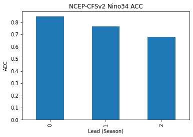
Compute the Anomaly Correlation Coefficient (ACC) climpred.metrics._pearson_r() for 0, 1, and 2 season lead-times.
skillds = hindcast.verify(
    metric="acc", comparison="e2o", dim="init", alignment="maximize"
)
skillds
<xarray.Dataset>
Dimensions:  (lead: 3)
Coordinates:
  * lead     (lead) int64 0 1 2
    skill    <U11 'initialized'
Data variables:
    sst      (lead) float64 0.8466 0.7671 0.6785
Attributes:
    prediction_skill_software:     climpred https://climpred.readthedocs.io/
    skill_calculated_by_function:  HindcastEnsemble.verify()
    number_of_initializations:     348
    alignment:                     maximize
    metric:                        pearson_r
    comparison:                    e2o
    dim:                           init
reference: []skillds.sst.to_series().plot(kind="bar")
plt.title("NCEP-CFSv2 Nino34 ACC")
plt.xlabel("Lead (Season)")
plt.ylabel("ACC")
plt.show()
Text(0, 0.5, 'ACC')
References
- 1
Ben P. Kirtman, Dughong Min, Johnna M. Infanti, James L. Kinter, Daniel A. Paolino, Qin Zhang, Huug van den Dool, Suranjana Saha, Malaquias Pena Mendez, Emily Becker, Peitao Peng, Patrick Tripp, Jin Huang, David G. DeWitt, Michael K. Tippett, Anthony G. Barnston, Shuhua Li, Anthony Rosati, Siegfried D. Schubert, Michele Rienecker, Max Suarez, Zhao E. Li, Jelena Marshak, Young-Kwon Lim, Joseph Tribbia, Kathleen Pegion, William J. Merryfield, Bertrand Denis, and Eric F. Wood. The North American Multimodel Ensemble: Phase-1 Seasonal-to-Interannual Prediction; Phase-2 toward Developing Intraseasonal Prediction. Bulletin of the American Meteorological Society, 95(4):585–601, April 2014. doi:10/ggspp9.