Hindcast Predictions of Equatorial Pacific SSTs¶

In this example, we evaluate hindcasts (retrospective forecasts) with HindcastEnsemble of sea surface temperatures in the eastern equatorial Pacific from CESM-DPLE. These hindcasts are evaluated against a forced ocean-sea ice simulation that initializes the model.

See the quick start for an analysis of time series (rather than maps) from HindcastEnsemble.

# linting
%load_ext nb_black
%load_ext lab_black

%matplotlib inline
import matplotlib.pyplot as plt
import numpy as np

import climpred
from climpred import HindcastEnsemble
import xarray as xr

xr.set_options(display_style="text")

# silence warnings if annoying
# import warnings
# warnings.filterwarnings("ignore")

<xarray.core.options.set_options at 0x10d603d30>

We’ll load in a small region of the eastern equatorial Pacific for this analysis example.

initialized = climpred.tutorial.load_dataset("CESM-DP-SST-3D")["SST"]
recon = climpred.tutorial.load_dataset("FOSI-SST-3D")["SST"]
initialized

<xarray.DataArray 'SST' (init: 64, lead: 10, nlat: 37, nlon: 26)>
[615680 values with dtype=float32]
Coordinates:
    TLAT     (nlat, nlon) float64 ...
    TLONG    (nlat, nlon) float64 ...
  * init     (init) float32 1.954e+03 1.955e+03 ... 2.016e+03 2.017e+03
  * lead     (lead) int32 1 2 3 4 5 6 7 8 9 10
    TAREA    (nlat, nlon) float64 ...
Dimensions without coordinates: nlat, nlon

These two example products cover a small portion of the eastern equatorial Pacific.

It is generally advisable to do all bias correction before instantiating a HindcastEnsemble. However, HindcastEnsemble can also be modified with HindcastEnsemble.remove_bias().

climpred requires that lead dimension has an attribute called units indicating what time units the lead is assocated with. Options are: years, seasons, months, weeks, pentads, days, hours, minutes, seconds. For the this data, the lead units are years.

initialized["lead"].attrs["units"] = "years"

hindcast = HindcastEnsemble(initialized).add_observations(recon)
hindcast

/Users/aaron.spring/Coding/climpred/climpred/utils.py:191: UserWarning: Assuming annual resolution starting Jan 1st due to numeric inits. Please change ``init`` to a datetime if it is another resolution. We recommend using xr.CFTimeIndex as ``init``, see https://climpred.readthedocs.io/en/stable/setting-up-data.html.
  warnings.warn(
/Users/aaron.spring/Coding/climpred/climpred/utils.py:191: UserWarning: Assuming annual resolution starting Jan 1st due to numeric inits. Please change ``init`` to a datetime if it is another resolution. We recommend using xr.CFTimeIndex as ``init``, see https://climpred.readthedocs.io/en/stable/setting-up-data.html.
  warnings.warn(

<climpred.HindcastEnsemble>
Initialized Ensemble:
    SST      (init, lead, nlat, nlon) float32 -0.3323 -0.3238 ... 1.179 1.123
Observations:
    SST      (time, nlat, nlon) float32 25.53 25.43 25.35 ... 27.03 27.1 27.05
Uninitialized:
    None

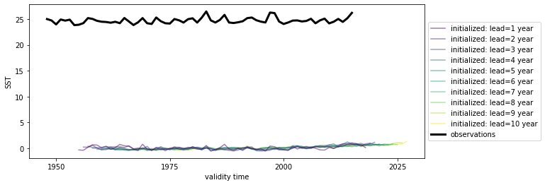
# Quick look at the HindEnsemble timeseries: only works for 1-dimensional data, therefore take spatial mean
hindcast.mean(["nlat", "nlon"]).plot()

<AxesSubplot:xlabel='validity time', ylabel='SST'>

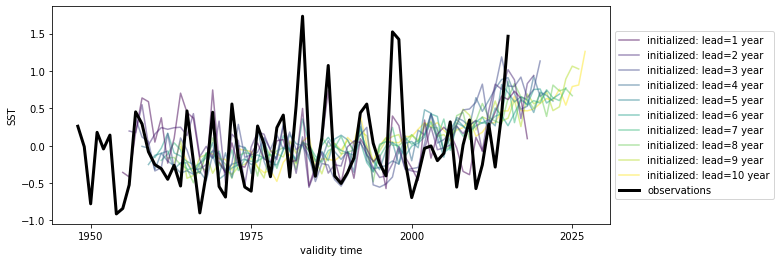
../../_images/tropical-pacific-ssts_11_1.png

We first need to remove the same climatology that was used to drift-correct the CESM-DPLE.

recon = recon - recon.sel(time=slice(1964, 2014)).mean("time")
hindcast = hindcast.add_observations(recon)
hindcast.mean(["nlat", "nlon"]).plot()

/Users/aaron.spring/Coding/climpred/climpred/utils.py:191: UserWarning: Assuming annual resolution starting Jan 1st due to numeric inits. Please change ``init`` to a datetime if it is another resolution. We recommend using xr.CFTimeIndex as ``init``, see https://climpred.readthedocs.io/en/stable/setting-up-data.html.
  warnings.warn(

<AxesSubplot:xlabel='validity time', ylabel='SST'>

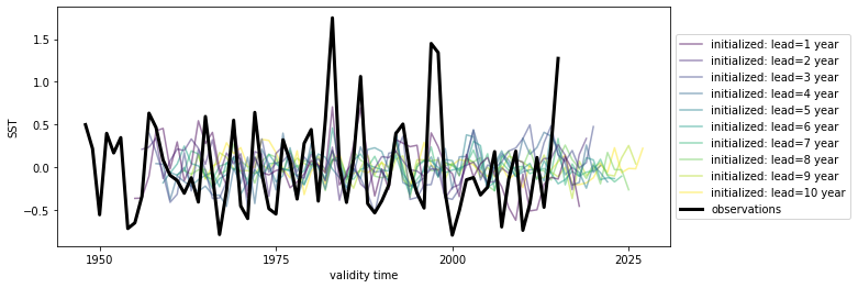
../../_images/tropical-pacific-ssts_13_2.png

We’ll also detrend climpred.stats.rm_trend() the reconstruction over its time dimension and initialized forecast ensemble over lead.

from climpred.stats import rm_trend

hindcast_detrend = hindcast.map(rm_trend, dim="lead_or_time")

hindcast_detrend.mean(["nlat", "nlon"]).plot()

<AxesSubplot:xlabel='validity time', ylabel='SST'>

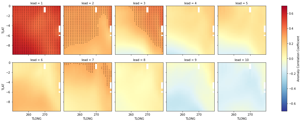
../../_images/tropical-pacific-ssts_16_1.png

Anomaly Correlation Coefficient of SSTs¶

We can now compute the ACC climpred.metrics._pearson_r() over all leads and all grid cells with HindcastEnsemble.verify.

predictability = hindcast_detrend.verify(
    metric="acc", comparison="e2o", dim="init", alignment="same_verif"
)
predictability

<xarray.Dataset>
Dimensions:  (lead: 10, nlat: 37, nlon: 26)
Coordinates:
  * nlat     (nlat) int64 0 1 2 3 4 5 6 7 8 9 ... 27 28 29 30 31 32 33 34 35 36
  * nlon     (nlon) int64 0 1 2 3 4 5 6 7 8 9 ... 16 17 18 19 20 21 22 23 24 25
    TLONG    (nlat, nlon) float64 250.8 251.9 253.1 254.2 ... 276.7 277.8 278.9
  * lead     (lead) int32 1 2 3 4 5 6 7 8 9 10
    TAREA    (nlat, nlon) float64 3.661e+13 3.661e+13 ... 3.714e+13 3.714e+13
    TLAT     (nlat, nlon) float64 -9.75 -9.75 -9.75 ... -0.1336 -0.1336 -0.1336
    skill    <U11 'initialized'
Data variables:
    SST      (lead, nlat, nlon) float64 0.6272 0.6248 ... -0.05417 -0.05513
Attributes:
    prediction_skill_software:     climpred https://climpred.readthedocs.io/
    skill_calculated_by_function:  HindcastEnsemble.verify()
    number_of_initializations:     64
    alignment:                     same_verif
    metric:                        pearson_r
    comparison:                    e2o
    dim:                           init
    reference:                     []

We use the pval keyword to get associated p-values for our ACCs. We can then mask our final maps based on $\alpha = 0.05$.

significance = hindcast_detrend.verify(
    metric="p_pval", comparison="e2o", dim="init", alignment="same_verif"
)

# Mask latitude and longitude by significance for stippling.
siglat = significance.TLAT.where(significance.SST <= 0.05)
siglon = significance.TLONG.where(significance.SST <= 0.05)

p = predictability.SST.plot.pcolormesh(
    x="TLONG",
    y="TLAT",
    col="lead",
    col_wrap=5,
    cbar_kwargs={"label": "Anomaly Correlation Coefficient"},
    vmin=-0.7,
    vmax=0.7,
    cmap="RdYlBu_r",
)
for i, ax in enumerate(p.axes.flat):
    # Add significance stippling
    ax.scatter(
        siglon.isel(lead=i), siglat.isel(lead=i), color="k", marker=".", s=1.5,
    )

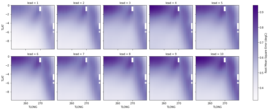
../../_images/tropical-pacific-ssts_21_0.png

Root Mean Square Error of SSTs¶

We can also check error in our forecasts, just by changing the metric keyword to _rmse() or _mae().

rmse = hindcast_detrend.verify(
    metric="rmse", comparison="e2o", dim="init", alignment="same_verif"
)

p = rmse.SST.plot.pcolormesh(
    x="TLONG",
    y="TLAT",
    col="lead",
    col_wrap=5,
    cbar_kwargs={"label": "Root Mean Square Error (degC)"},
    cmap="Purples",
)

../../_images/tropical-pacific-ssts_24_0.png

climpred documentation

Hindcast Predictions of Equatorial Pacific SSTs¶

Anomaly Correlation Coefficient of SSTs¶

Root Mean Square Error of SSTs¶