Calculate Seasonal ENSO Skill of the NMME model NCEP-CFSv2

In this example, we demonstrate:

1. How to remotely access data from the North American Multi-model Ensemble (NMME) hindcast database and set it up to be used in climpred

2. How to calculate the Anomaly Correlation Coefficient (ACC) using seasonal data

The North American Multi-model Ensemble (NMME)

Further information on NMME is available from Kirtman et al. 2014 and the NMME project website

The NMME public database is hosted on the International Research Institute for Climate and Society (IRI) data server http://iridl.ldeo.columbia.edu/SOURCES/.Models/.NMME/

Definitions

Anomalies

Departure from normal, where normal is defined as the climatological value based on the average value for each month over all years.

Nino3.4

An index used to represent the evolution of the El Nino-Southern Oscillation (ENSO). Calculated as the average sea surface temperature (SST) anomalies in the region 5S-5N; 190-240

import matplotlib.pyplot as plt
import xarray as xr
import pandas as pd
import numpy as np

from climpred import HindcastEnsemble
import climpred

def decode_cf(ds, time_var):
    """Decodes time dimension to CFTime standards."""
    if ds[time_var].attrs['calendar'] == '360':
        ds[time_var].attrs['calendar'] = '360_day'
    ds = xr.decode_cf(ds, decode_times=True)
    return ds

Load the monthly sea surface temperature (SST) hindcast data for the NCEP-CFSv2 model from the data server

# Get NMME data for NCEP-CFSv2, SST
url = 'http://iridl.ldeo.columbia.edu/SOURCES/.Models/.NMME/NCEP-CFSv2/.HINDCAST/.MONTHLY/.sst/dods'
fcstds = xr.open_dataset(url, decode_times=False, chunks={'S': 1, 'L': 12})
fcstds = decode_cf(fcstds, 'S')
fcstds

<xarray.Dataset>
Dimensions:  (L: 10, M: 24, S: 348, X: 360, Y: 181)
Coordinates:
  * S        (S) object 1982-01-01 00:00:00 ... 2010-12-01 00:00:00
  * M        (M) float32 1.0 2.0 3.0 4.0 5.0 6.0 ... 20.0 21.0 22.0 23.0 24.0
  * X        (X) float32 0.0 1.0 2.0 3.0 4.0 ... 355.0 356.0 357.0 358.0 359.0
  * L        (L) float32 0.5 1.5 2.5 3.5 4.5 5.5 6.5 7.5 8.5 9.5
  * Y        (Y) float32 -90.0 -89.0 -88.0 -87.0 -86.0 ... 87.0 88.0 89.0 90.0
Data variables:
    sst      (S, L, M, Y, X) float32 dask.array<chunksize=(1, 10, 24, 181, 360), meta=np.ndarray>
Attributes:
    Conventions:  IRIDL

The NMME data dimensions correspond to the following climpred dimension definitions: X=lon,L=lead,Y=lat,M=member, S=init. We will rename the dimensions to their climpred names.

fcstds=fcstds.rename({'S': 'init',
                      'L': 'lead',
                      'M': 'member',
                      'X': 'lon',
                      'Y': 'lat'})

Let’s make sure that the lead dimension is set properly for climpred. NMME data stores leads as 0.5, 1.5, 2.5, etc, which correspond to 0, 1, 2, … months since initialization. We will change the lead to be integers starting with zero.

fcstds['lead'] = (fcstds['lead'] - 0.5).astype('int')

Next, we want to get the verification SST data from the data server

obsurl='http://iridl.ldeo.columbia.edu/SOURCES/.Models/.NMME/.OIv2_SST/.sst/dods'
verifds = decode_cf(xr.open_dataset(obsurl, decode_times=False),'T')
verifds

<xarray.Dataset>
Dimensions:  (T: 405, X: 360, Y: 181)
Coordinates:
  * T        (T) object 1982-01-16 00:00:00 ... 2015-09-16 00:00:00
  * Y        (Y) float32 -90.0 -89.0 -88.0 -87.0 -86.0 ... 87.0 88.0 89.0 90.0
  * X        (X) float32 0.0 1.0 2.0 3.0 4.0 ... 355.0 356.0 357.0 358.0 359.0
Data variables:
    sst      (T, Y, X) float32 ...
Attributes:
    Conventions:  IRIDL

Rename the dimensions to correspond to climpred dimensions

verifds = verifds.rename({'T': 'time',
                          'X': 'lon',
                          'Y': 'lat'})

Convert the time data to be on the first of the month and in the same calendar format as the forecast output. The time dimension is natively decoded to start in February, even though it starts in January. It is also labelled as mid-month, and we need to label it as the start of the month to ensure that the dates align properly.

verifds['time'] = xr.cftime_range(start='1982-01', periods=verifds['time'].size, freq='MS', calendar='360_day')

Subset the data to 1982-2010

verifds = verifds.sel(time=slice('1982-01-01', '2010-12-01'))
fcstds = fcstds.sel(init=slice('1982-01-01', '2010-12-01'))

Calculate the Nino3.4 index for forecast and verification

fcstnino34=fcstds.sel(lat=slice(-5, 5), lon=slice(190, 240)).mean(['lat','lon'])
verifnino34=verifds.sel(lat=slice(-5, 5), lon=slice(190, 240)).mean(['lat','lon'])

fcstclimo = fcstnino34.groupby('init.month').mean('init')
fcstanoms = (fcstnino34.groupby('init.month') - fcstclimo)

verifclimo = verifnino34.groupby('time.month').mean('time')
verifanoms = (verifnino34.groupby('time.month') - verifclimo)

print(fcstanoms)
print(verifanoms)

<xarray.Dataset>
Dimensions:  (init: 348, lead: 10, member: 24)
Coordinates:
  * member   (member) float32 1.0 2.0 3.0 4.0 5.0 ... 20.0 21.0 22.0 23.0 24.0
  * lead     (lead) int64 0 1 2 3 4 5 6 7 8 9
  * init     (init) object 1982-01-01 00:00:00 ... 2010-12-01 00:00:00
    month    (init) int64 1 2 3 4 5 6 7 8 9 10 11 ... 2 3 4 5 6 7 8 9 10 11 12
Data variables:
    sst      (init, lead, member) float32 dask.array<chunksize=(1, 10, 24), meta=np.ndarray>
<xarray.Dataset>
Dimensions:  (time: 348)
Coordinates:
  * time     (time) object 1982-01-01 00:00:00 ... 2010-12-01 00:00:00
    month    (time) int64 1 2 3 4 5 6 7 8 9 10 11 ... 2 3 4 5 6 7 8 9 10 11 12
Data variables:
    sst      (time) float32 0.14492226 -0.044160843 ... -1.5685654 -1.6083965

Make Seasonal Averages with center=True and drop NaNs.

%%time
fcstnino34seas = fcstanoms.rolling(lead=3, center=True).mean().dropna(dim='lead')
verifnino34seas = verifanoms.rolling(time=3, center=True).mean().dropna(dim='time')

CPU times: user 4.31 s, sys: 2.29 s, total: 6.6 s
Wall time: 2min 23s

Create new xr.DataArray with seasonal data

# Grab only every three months, which center the seasonal averages.
nleads = fcstnino34seas['lead'].isel(lead=slice(0, None, 3)).size
fcst = xr.DataArray(fcstnino34seas['sst'].isel(lead=slice(0, None, 3)),
                    coords={'init' : fcstnino34seas['init'],
                            'lead': np.arange(0, nleads),
                            'member': fcstanoms['member'],
                            },
                    dims=['init','lead','member'])
fcst = fcst.rename('sst')

Assign the units attribute of seasons to the lead dimension, which will align leads based on 3-month increments.

fcst['lead'].attrs = {'units': 'seasons'}

Create a climpred HindcastEnsemble object

hindcast = HindcastEnsemble(fcst)
hindcast = hindcast.add_observations(verifnino34seas)

Compute the Anomaly Correlation Coefficient (ACC) 0, 1, 2, and 3 season lead-times

skillds = hindcast.verify(metric='acc', comparison='e2o', dim='init', alignment='maximize')
skillds

<xarray.Dataset>
Dimensions:  (lead: 3, skill: 1)
Coordinates:
  * lead     (lead) int64 0 1 2
  * skill    (skill) <U4 'init'
Data variables: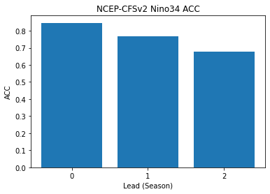
    sst      (lead) float64 0.8466 0.7672 0.6786

Make bar plot of Nino3.4 skill for 0,1, and 2 season lead times

x=np.arange(0,nleads,1.0).astype(int)
plt.bar(x,skillds['sst'])
plt.xticks(x)
plt.title('NCEP-CFSv2 Nino34 ACC')
plt.xlabel('Lead (Season)')
plt.ylabel('ACC')

Text(0, 0.5, 'ACC')

References

1. Kirtman, B.P., D. Min, J.M. Infanti, J.L. Kinter, D.A. Paolino, Q. Zhang, H. van den Dool, S. Saha, M.P. Mendez, E. Becker, P. Peng, P. Tripp, J. Huang, D.G. DeWitt, M.K. Tippett, A.G. Barnston, S. Li, A. Rosati, S.D. Schubert, M. Rienecker, M. Suarez, Z.E. Li, J. Marshak, Y. Lim, J. Tribbia, K. Pegion, W.J. Merryfield, B. Denis, and E.F. Wood, 2014: The North American Multimodel Ensemble: Phase-1 Seasonal-to-Interannual Prediction; Phase-2 toward Developing Intraseasonal Prediction. Bull. Amer. Meteor. Soc., 95, 585–601, https://doi.org/10.1175/BAMS-D-12-00050.1