climpred.metrics._spearman_r_eff_p_value
- climpred.metrics._spearman_r_eff_p_value(forecast, verif, dim=None, **metric_kwargs)[source]
Probability that forecast and verification data are monotonically uncorrelated, accounting for autocorrelation.
Note
Weights are not included here due to the dependence on temporal autocorrelation.
Note
This metric can only be used for hindcast-type simulations.
The effective p value is computed by replacing the sample size
 in the
t-statistic with the effective sample size,
in the
t-statistic with the effective sample size,  . The same Spearman’s
rank correlation coefficient
. The same Spearman’s
rank correlation coefficient  is used as when computing the standard p
value.
is used as when computing the standard p
value.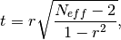
where
is computed via the autocorrelation in the forecast and
verification data.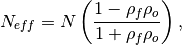
where
 and
and  are the lag-1 autocorrelation
coefficients for the forecast and verification data.
are the lag-1 autocorrelation
coefficients for the forecast and verification data.- Parameters
forecast (xarray object) – Forecast.
verif (xarray object) – Verification data.
dim (str) – Dimension(s) to perform metric over.
metric_kwargs (dict) – see
spearman_r_eff_p_value()
- Details:
minimum
0.0
maximum
1.0
perfect
1.0
orientation
negative
- Reference:
Bretherton, Christopher S., et al. “The effective number of spatial degrees of freedom of a time-varying field.” Journal of climate 12.7 (1999): 1990-2009.
Example
>>> HindcastEnsemble.verify(metric='spearman_r_eff_p_value', comparison='e2o',
...     alignment='same_verifs', dim='init')
<xarray.Dataset>
Dimensions:  (lead: 10)
Coordinates:
  * lead     (lead) int32 1 2 3 4 5 6 7 8 9 10
    skill    <U11 'initialized'
Data variables:
    SST      (lead) float64 0.02034 0.0689 0.2408 ... 0.2092 0.2315 0.2347