climpred.metrics._effective_sample_size¶

climpred.metrics._effective_sample_size(forecast, verif, dim=None, **metric_kwargs)[source]¶

Effective sample size for temporally correlated data.

Note

Weights are not included here due to the dependence on temporal autocorrelation.

Note

This metric can only be used for hindcast-type simulations.

The effective sample size extracts the number of independent samples between two time series being correlated. This is derived by assessing the magnitude of the lag-1 autocorrelation coefficient in each of the time series being correlated. A higher autocorrelation induces a lower effective sample size which raises the correlation coefficient for a given p value.

The effective sample size is used in computing the effective p value. See pearson_r_eff_p_value and spearman_r_eff_p_value.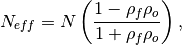

$N_{eff} = N\left( \frac{1 - \rho_{f}\rho_{o}}{1 + \rho_{f}\rho_{o}} \right),$

where $\rho_{f}$ and $\rho_{o}$ are the lag-1 autocorrelation coefficients for the forecast and verification data.

Parameters

forecast (xarray object) – Forecast.
verif (xarray object) – Verification data.
dim (str) – Dimension(s) to perform metric over.
metric_kwargs (dict) – see effective_sample_size()

Details:

minimum	0.0
maximum	∞
perfect	N/A
orientation	positive

Reference:

Bretherton, Christopher S., et al. “The effective number of spatial degrees of freedom of a time-varying field.” Journal of climate 12.7 (1999): 1990-2009.

Example

>>> HindcastEnsemble.verify(metric='effective_sample_size', comparison='e2o',
...     alignment='same_verifs', dim='init')
<xarray.Dataset>
Dimensions:  (lead: 10)
Coordinates:
  * lead     (lead) int32 1 2 3 4 5 6 7 8 9 10
    skill    <U11 'initialized'
Data variables:
    SST      (lead) float64 5.0 4.0 3.0 3.0 3.0 3.0 3.0 3.0 3.0 3.0