Temporal and Spatial Smoothing
This demo demonstrates climpred’s capabilities to postprocess decadal prediction output before skill verification. Here, we showcase a set of methods to smooth out noise in the spatial and temporal domain.
[1]:
import warnings
%matplotlib inline
from climpred import PerfectModelEnsemble, HindcastEnsemble
from climpred.tutorial import load_dataset
import matplotlib.pylab as plt
warnings.filterwarnings("ignore")
import xarray as xr

xr.set_options(display_style='text')
[1]:
<xarray.core.options.set_options at 0x7fbf31daaba8>
[2]:
# Sea surface temperature
v='tos'
ds3d = load_dataset('MPI-PM-DP-3D')[v]
control3d = load_dataset('MPI-control-3D')[v]
climpred requires that lead dimension has an attribute called units indicating what time units the lead is assocated with. Options are: years, seasons, months, weeks, pentads, days. For the this data, the lead units are years.
[3]:
ds3d['lead'].attrs={'units': 'years'}
Temporal smoothing
In order to reduce temporal noise, decadal predictions are recommended to take multi-year averages [Goddard2013].
[4]:
pm = PerfectModelEnsemble(ds3d)
pm = pm.add_control(control3d)
PredictionEnsemble.smooth({'lead':x}) aggregates over x timesteps in time dimensions lead and time. Here it does not matter whether you specify lead or time, temporal smoothing is applied to both time dimensions. Note that the time dimension labels are not changed by this temporal smoothing.
[5]:
pm_tsmoothed = pm.smooth({'lead':3})
print('initialized', pm_tsmoothed.get_initialized().coords,'\n')
print('control',pm_tsmoothed.get_control().coords)
initialized Coordinates:
    lon      (y, x) float64 ...
    lat      (y, x) float64 ...
  * lead     (lead) int64 1 2 3
  * init     (init) object 3014-01-01 00:00:00 ... 3237-01-01 00:00:00
  * member   (member) int64 1 2 3 4

control Coordinates:
    lon      (y, x) float64 ...
    lat      (y, x) float64 ...
  * time     (time) object 3000-01-01 00:00:00 ... 3047-01-01 00:00:00
But after calling verify(), the correct time aggregation label is automatically set.
[6]:
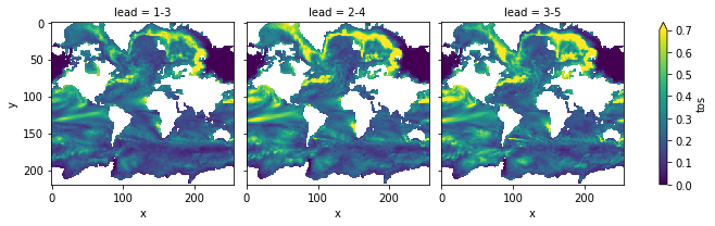
pm_tsmoothed.verify(metric='rmse',
                    comparison='m2e',
                    dim=['init', 'member'])[v] \
            .plot(col='lead', vmin=0, vmax=.7, yincrease=False, x='x')
[6]:
<xarray.plot.facetgrid.FacetGrid at 0x7fbf39391dd8>
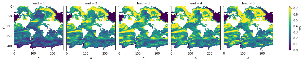
Compare to the prediction skill without smoothing:
[7]:
pm.verify(metric='rmse',
          comparison='m2e',
          dim=['init','member'])[v] \
   .plot(col='lead', vmin=0, vmax=.7, yincrease=False, x='x')
[7]:
<xarray.plot.facetgrid.FacetGrid at 0x7fbf1dcf54a8>
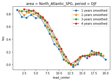
You can plot time-aggregated skill timeseries by specifying x=lead_center while plotting. Lead centers are placed in the center of the lead-aggregation boundaries. Note how the correlation of forecasts is increasing for longer time-aggregations because noise is smoothed out.
[8]:
pm_NA = PerfectModelEnsemble(load_dataset('MPI-PM-DP-1D').tos)
pm_NA = pm_NA.add_control(load_dataset('MPI-control-1D').tos)
pm_NA = pm_NA.sel(area='North_Atlantic_SPG',period='DJF')
[9]:
for time_agg in [1,2,3,4]:
    pm_NA.smooth({'lead':time_agg}).verify(metric='acc', comparison='m2e', dim=['init','member']).tos.plot(
        x='lead_center', marker='o',label=f'{time_agg}-years smoothed')
plt.legend()
[9]:
<matplotlib.legend.Legend at 0x7fbf1fc97d30>
Now, we showcase these features for a HindcastEnsemble.
[10]:
v='SST'
hind = load_dataset('CESM-DP-SST-3D')[v]
reconstruction = load_dataset('FOSI-SST-3D')[v]
# Move reconstruction into proper anomaly space
reconstruction = reconstruction - reconstruction.sel(time=slice(1964, 2014)).mean('time')
[11]:
hindcast = HindcastEnsemble(hind)
hindcast = hindcast.add_observations(reconstruction)
[12]:
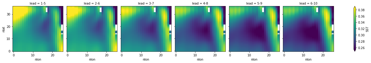
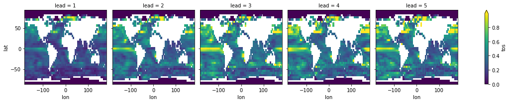
hindcast.smooth({'lead': 5}) \
        .verify(metric='rmse',
                comparison='e2r',
                dim='init',
                alignment='same_verif')[v] \
        .plot(col='lead', robust=True)
[12]:
<xarray.plot.facetgrid.FacetGrid at 0x7fbf1ef443c8>
Spatial smoothing
In order to reduce spatial noise, global decadal predictions are recommended to get regridded to a 5 degree longitude x 5 degree latitude grid as recommended [Goddard2013].
[13]:
v='tos'
pm_ssmoothed = pm.smooth({'lon':5,'lat':5})
pm_ssmoothed.get_initialized().coords
Reuse existing file: bilinear_220x256_36x73.nc
Reuse existing file: bilinear_220x256_36x73.nc
[13]:
Coordinates:
  * lead     (lead) int64 1 2 3 4 5
  * init     (init) object 3014-01-01 00:00:00 ... 3237-01-01 00:00:00
  * member   (member) int64 1 2 3 4
  * lon      (lon) float64 -180.0 -175.0 -170.0 -165.0 ... 170.0 175.0 180.0
  * lat      (lat) float64 -83.97 -78.97 -73.97 -68.97 ... 81.03 86.03 91.03
[14]:
pm_ssmoothed.verify(metric='rmse',
                    comparison='m2e',
                    dim=['init', 'member'])[v] \
            .plot(col='lead', robust=True, yincrease=True)
[14]:
<xarray.plot.facetgrid.FacetGrid at 0x7fbf1ee92c88>
Spatial smoothing guesses the names corresponding to lon and lat in the coordinates of the PredictionEnsemble underlying datasets.
[15]:
hindcast.get_initialized().coords
[15]:
Coordinates:
    TLAT     (nlat, nlon) float64 ...
    TLONG    (nlat, nlon) float64 ...
  * init     (init) object 1954-01-01 00:00:00 ... 2017-01-01 00:00:00
  * lead     (lead) int32 1 2 3 4 5 6 7 8 9 10
    TAREA    (nlat, nlon) float64 ...
[16]:
hindcast.smooth({'lon':1, 'lat':1}).get_initialized().coords
Reuse existing file: bilinear_37x26_11x30.nc
Reuse existing file: bilinear_37x26_11x30.nc
[16]:
Coordinates:
  * init     (init) object 1954-01-01 00:00:00 ... 2017-01-01 00:00:00
  * lead     (lead) int32 1 2 3 4 5 6 7 8 9 10
  * lon      (lon) float64 250.8 251.8 252.8 253.8 ... 276.8 277.8 278.8 279.8
  * lat      (lat) float64 -9.75 -8.75 -7.75 -6.75 ... -1.75 -0.7503 0.2497
PredictionEnsemble.smooth(goddard2013) creates 4-year means and 5x5 degree regridding as suggested in [Goddard2013].
[17]:
pm.smooth('goddard2013') \
  .verify(metric='acc',
          comparison='m2e',
          dim=['init','member']).coords
Reuse existing file: bilinear_220x256_36x73.nc
Reuse existing file: bilinear_220x256_36x73.nc
[17]:
Coordinates:
  * lead         (lead) <U3 '1-4' '2-5'
  * lon          (lon) float64 -180.0 -175.0 -170.0 -165.0 ... 170.0 175.0 180.0
  * lat          (lat) float64 -83.97 -78.97 -73.97 -68.97 ... 81.03 86.03 91.03
    lead_center  (lead) float64 2.5 3.5
References
Goddard, L., A. Kumar, A. Solomon, D. Smith, G. Boer, P. Gonzalez, V. Kharin, et al. “A Verification Framework for Interannual-to-Decadal Predictions Experiments.” Climate Dynamics 40, no. 1–2 (January 1, 2013): 245–72. https://doi.org/10/f4jjvf.