PredictionEnsemble Objects
One of the major features of climpred is our objects that are based upon the PredictionEnsemble class. We supply users with a HindcastEnsemble and PerfectModelEnsemble object. We encourage users to take advantage of these high-level objects, which wrap all of our core functions. These objects don’t comprehensively cover all functions yet, but eventually we’ll deprecate direct access to the function calls in favor of the lightweight objects.
Briefly, we consider a HindcastEnsemble to be one that is initialized from some observational-like product (e.g., assimilated data, reanalysis products, or a model reconstruction). Thus, this object is built around comparing the initialized ensemble to various observational products. In contrast, a PerfectModelEnsemble is one that is initialized off of a model control simulation. These forecasting systems are not meant to be compared directly to real-world observations. Instead, they
provide a contained model environment with which to theoretically study the limits of predictability. You can read more about the terminology used in climpred here.
Let’s create a demo object to explore some of the functionality and why they are much smoother to use than direct function calls.
[1]:
%matplotlib inline
import matplotlib.pyplot as plt
import xarray as xr

from climpred import HindcastEnsemble
import climpred
We can pull in some sample data that is packaged with climpred.
[2]:
climpred.tutorial.load_dataset()
'MPI-control-1D': area averages for the MPI control run of SST/SSS.
'MPI-control-3D': lat/lon/time for the MPI control run of SST/SSS.
'MPI-PM-DP-1D': perfect model decadal prediction ensemble area averages of SST/SSS/AMO.
'MPI-PM-DP-3D': perfect model decadal prediction ensemble lat/lon/time of SST/SSS/AMO.
'CESM-DP-SST': hindcast decadal prediction ensemble of global mean SSTs.
'CESM-DP-SSS': hindcast decadal prediction ensemble of global mean SSS.
'CESM-DP-SST-3D': hindcast decadal prediction ensemble of eastern Pacific SSTs.
'CESM-LE': uninitialized ensemble of global mean SSTs.
'MPIESM_miklip_baseline1-hind-SST-global': hindcast initialized ensemble of global mean SSTs
'MPIESM_miklip_baseline1-hist-SST-global': uninitialized ensemble of global mean SSTs
'MPIESM_miklip_baseline1-assim-SST-global': assimilation in MPI-ESM of global mean SSTs
'ERSST': observations of global mean SSTs.
'FOSI-SST': reconstruction of global mean SSTs.
'FOSI-SSS': reconstruction of global mean SSS.
'FOSI-SST-3D': reconstruction of eastern Pacific SSTs
'GMAO-GEOS-RMM1': daily RMM1 from the GMAO-GEOS-V2p1 model for SubX
'RMM-INTERANN-OBS': observed RMM with interannual variablity included
HindcastEnsemble
We’ll start out with a HindcastEnsemble demo, followed by a PerfectModelEnsemble case.
[3]:
hind = climpred.tutorial.load_dataset('CESM-DP-SST') # CESM-DPLE hindcast ensemble output.
obs = climpred.tutorial.load_dataset('ERSST') # ERSST observations.
recon = climpred.tutorial.load_dataset('FOSI-SST') # Reconstruction simulation that initialized CESM-DPLE.
We need to add a “units” attribute to the hindcast ensemble so that climpred knows how to interpret the lead units.
[4]:
hind["lead"].attrs["units"] = "years"
CESM-DPLE was drift-corrected prior to uploading the output, so we just need to subtract the climatology over the same period for our other products before building the object.
[5]:
obs = obs - obs.sel(time=slice(1964, 2014)).mean('time')
recon = recon - recon.sel(time=slice(1964, 2014)).mean('time')
Now we instantiate the HindcastEnsemble object and append all of our products to it.
[6]:
hindcast = HindcastEnsemble(hind) # Instantiate object by passing in our initialized ensemble.
print(hindcast)
<climpred.HindcastEnsemble>
Initialized Ensemble:
    SST      (init, lead, member) float64 ...
Observationss:
    None
Uninitialized:
    None
/Users/ribr5703/miniconda3/envs/climpred-dev/lib/python3.6/site-packages/climpred/utils.py:48: UserWarning: Assuming annual resolution due to numeric inits. Change init to a datetime if it is another resolution.
  'Assuming annual resolution due to numeric inits. '
Now we just use the add_ methods to attach other objects. See the API here. Note that we strive to make our conventions follow those of ``xarray``’s. For example, we don’t allow inplace operations. One has to run hindcast = hindcast.add_observations(...) to modify the object upon later calls rather than just hindcast.add_observations(...).
[7]:
hindcast = hindcast.add_observations(recon, 'reconstruction')
hindcast = hindcast.add_observations(obs, 'ERSST')
[8]:
print(hindcast)
<climpred.HindcastEnsemble>
Initialized Ensemble:
    SST      (init, lead, member) float64 ...
reconstruction:
    SST      (time) float64 -0.05064 -0.0868 -0.1396 ... 0.3023 0.3718 0.292
ERSST:
    SST      (time) float32 -0.40146065 -0.35238647 ... 0.34601402 0.45021248
Uninitialized:
    None
You can apply most standard xarray functions directly to our objects! climpred will loop through the objects and apply the function to all applicable xarray.Datasets within the object. If you reference a dimension that doesn’t exist for the given xarray.Dataset, it will ignore it. This is useful, since the initialized ensemble is expected to have dimension init, while other products have dimension time (see more here).
Let’s start by taking the ensemble mean of the initialized ensemble so our metric computations don’t have to take the extra time on that later. I’m just going to use deterministic metrics here, so we don’t need the individual ensemble members. Note that above our initialized ensemble had a member dimension, and now it is reduced.
[9]:
hindcast = hindcast.mean('member')
print(hindcast)
<climpred.HindcastEnsemble>
Initialized Ensemble:
    SST      (init, lead) float64 -0.2121 -0.1637 -0.1206 ... 0.7286 0.7532
reconstruction:
    SST      (time) float64 -0.05064 -0.0868 -0.1396 ... 0.3023 0.3718 0.292
ERSST:
    SST      (time) float32 -0.40146065 -0.35238647 ... 0.34601402 0.45021248
Uninitialized:
    None
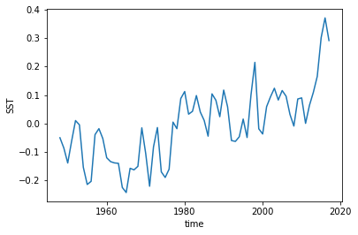
We still have a trend in all of our products, so we could also detrend them as well.
[10]:
hindcast.get_observations('reconstruction').SST.plot()
[10]:
[<matplotlib.lines.Line2D at 0x7fce880c2630>]
[11]:
from scipy.signal import detrend
I’m going to transpose this first since my initialized ensemble has dimensions ordered (init, lead) and scipy.signal.detrend is applied over the last axis. I’d like to detrend over the init dimension rather than lead dimension.
[12]:
hindcast = hindcast.transpose().apply(detrend)
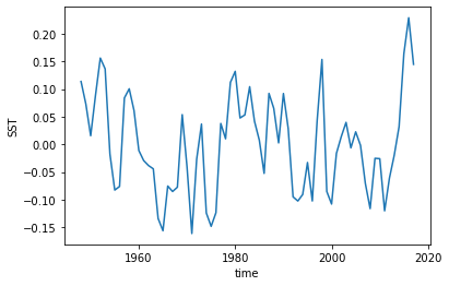
And it looks like everything got detrended by a linear fit! That wasn’t too hard.
[13]:
hindcast.get_observations('reconstruction').SST.plot()
[13]:
[<matplotlib.lines.Line2D at 0x7fceb8faa048>]
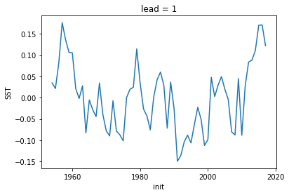
[14]:
hindcast.get_initialized().isel(lead=0).SST.plot()
[14]:
[<matplotlib.lines.Line2D at 0x7fce7a279e10>]
Now that we’ve done our pre-processing, let’s quickly compute some metrics. Check the metrics page here for all the keywords you can use. The API is currently pretty simple for the HindcastEnsemble. You can essentially compute standard skill metrics and a reference persistence forecast.
If you just pass a metric, it’ll compute the skill metric against all observations and return a dictionary with keys of the names the user entered when adding them.
[15]:
hindcast.verify(metric='mse')
[15]:
{'reconstruction': <xarray.Dataset>
 Dimensions:  (lead: 10)
 Coordinates:
   * lead     (lead) int32 1 2 3 4 5 6 7 8 9 10
 Data variables:
     SST      (lead) float64 0.005091 0.009096 0.008964 ... 0.01103 0.01261
 Attributes:
     prediction_skill:              calculated by climpred https://climpred.re...
     skill_calculated_by_function:  compute_hindcast
     number_of_initializations:     64
     metric:                        mse
     comparison:                    e2o
     dim:                           time
     created:                       2020-01-21 11:46:51,
 'ERSST': <xarray.Dataset>
 Dimensions:  (lead: 10)
 Coordinates:
   * lead     (lead) int32 1 2 3 4 5 6 7 8 9 10
 Data variables:
     SST      (lead) float64 0.003606 0.005651 0.006373 ... 0.007823 0.009009
 Attributes:
     prediction_skill:              calculated by climpred https://climpred.re...
     skill_calculated_by_function:  compute_hindcast
     number_of_initializations:     64
     metric:                        mse
     comparison:                    e2o
     dim:                           time
     created:                       2020-01-21 11:46:51}
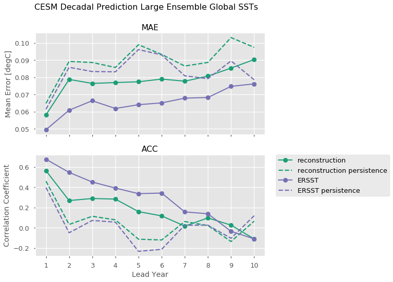
One can also directly call individual observations to compare to. Here we leverage xarray’s plotting method to compute Mean Absolute Error and the Anomaly Correlation Coefficient for both our observational products, as well as the equivalent metrics computed for persistence forecasts for each of those metrics.
[16]:
import numpy as np

plt.style.use('ggplot')
plt.style.use('seaborn-talk')

RECON_COLOR = '#1b9e77'
OBS_COLOR = '#7570b3'

f, axs = plt.subplots(nrows=2, figsize=(8, 8), sharex=True)

for ax, metric in zip(axs.ravel(), ['mae', 'acc']):
    handles = []
    for product, color in zip(['reconstruction', 'ERSST'], [RECON_COLOR, OBS_COLOR]):
        p1, = hindcast.verify(product, metric=metric).SST.plot(ax=ax,
                                                               marker='o',
                                                               color=color,
                                                               label=product,
                                                               linewidth=2)
        p2, = hindcast.compute_persistence(product, metric=metric).SST.plot(ax=ax,
                                                                      color=color,
                                                                      linestyle='--',
                                                                      label=product + ' persistence')
        handles.append(p1)
        handles.append(p2)
    ax.set_title(metric.upper())


axs[0].set_ylabel('Mean Error [degC]')
axs[1].set_ylabel('Correlation Coefficient')
axs[0].set_xlabel('')
axs[1].set_xlabel('Lead Year')
axs[1].set_xticks(np.arange(10)+1)

# matplotlib/xarray returning weirdness for the legend handles.
handles = [i.get_label() for i in handles]

# a little trick to put the legend on the outside.
plt.legend(handles, bbox_to_anchor=(1.05, 1), loc=2, borderaxespad=0.0)

plt.suptitle('CESM Decadal Prediction Large Ensemble Global SSTs', fontsize=16)
plt.show()
PerfectModelEnsemble
We’ll now play around a bit with the PerfectModelEnsemble object, using sample data from the MPI perfect model configuration.
[17]:
from climpred import PerfectModelEnsemble
[18]:
ds = climpred.tutorial.load_dataset('MPI-PM-DP-1D') # initialized ensemble from MPI
control = climpred.tutorial.load_dataset('MPI-control-1D') # base control run that initialized it
[19]:
ds["lead"].attrs["units"] = "years"
[20]:
print(ds)
<xarray.Dataset>
Dimensions:  (area: 3, init: 12, lead: 20, member: 10, period: 5)
Coordinates:
  * lead     (lead) int64 1 2 3 4 5 6 7 8 9 10 11 12 13 14 15 16 17 18 19 20
  * period   (period) object 'DJF' 'JJA' 'MAM' 'SON' 'ym'
  * area     (area) object 'global' 'North_Atlantic' 'North_Atlantic_SPG'
  * init     (init) int64 3014 3023 3045 3061 3124 ... 3175 3178 3228 3237 3257
  * member   (member) int64 0 1 2 3 4 5 6 7 8 9
Data variables:
    tos      (period, lead, area, init, member) float32 ...
    sos      (period, lead, area, init, member) float32 ...
    AMO      (period, lead, area, init, member) float32 ...
[21]:
pm = climpred.PerfectModelEnsemble(ds)
pm = pm.add_control(control)
print(pm)
<climpred.PerfectModelEnsemble>
Initialized Ensemble:
    tos      (period, lead, area, init, member) float32 ...
    sos      (period, lead, area, init, member) float32 ...
    AMO      (period, lead, area, init, member) float32 ...
Control:
    tos      (period, time, area) float32 ...
    sos      (period, time, area) float32 ...
    AMO      (period, time, area) float32 ...
Uninitialized:
    None
/Users/ribr5703/miniconda3/envs/climpred-dev/lib/python3.6/site-packages/climpred/utils.py:48: UserWarning: Assuming annual resolution due to numeric inits. Change init to a datetime if it is another resolution.
  'Assuming annual resolution due to numeric inits. '
Our objects are carrying sea surface temperature (tos), sea surface salinity (sos), and the Atlantic Multidecadal Oscillation index (AMO). Say we just want to look at skill metrics for temperature and salinity over the North Atlantic in JJA. We can just call a few easy xarray commands to filter down our object.
[22]:
pm = pm.drop('AMO').sel(area='North_Atlantic', period='JJA')
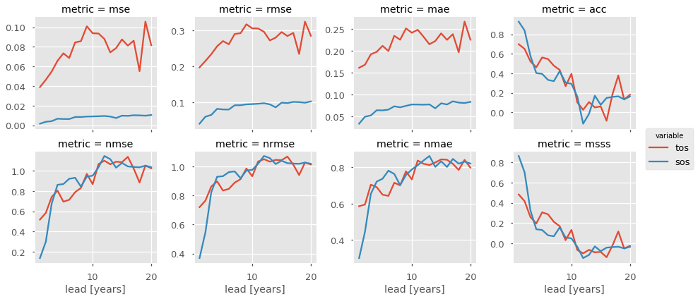
Now we can easily compute for a host of metrics. Here I just show a number of deterministic skill metrics comparing all individual members to the initialized ensemble mean. See comparisons for more information on the comparison keyword.
[23]:
METRICS = ['mse', 'rmse', 'mae', 'acc',
           'nmse', 'nrmse', 'nmae', 'msss']

result = []
for metric in METRICS:
    result.append(pm.compute_metric(metric, comparison='m2e'))

result = xr.concat(result, 'metric')
result['metric'] = METRICS

# Leverage the `xarray` plotting wrapper to plot all results at once.
result.to_array().plot(col='metric',
                       hue='variable',
                       col_wrap=4,
                       sharey=False,
                       sharex=True)
[23]:
<xarray.plot.facetgrid.FacetGrid at 0x7fcec93364e0>
It is useful to compare the initialized ensemble to an uninitialized run. See terminology for a description on “uninitialized” simulations. This gives us information about how initializations lead to enhanced predictability over knowledge of external forcing, whereas a comparison to persistence just tells us how well a dynamical forecast simulation does in comparison to a naive method. We can use the generate_uninitialized() method to bootstrap the control run and
create a pseudo-ensemble that approximates what an uninitialized ensemble would look like.
[24]:
pm = pm.generate_uninitialized()
print(pm)
<climpred.PerfectModelEnsemble>
Initialized Ensemble:
    tos      (lead, init, member) float32 ...
    sos      (lead, init, member) float32 ...
Control:
    tos      (time) float32 ...
    sos      (time) float32 ...
Uninitialized:
    tos      (init, member, lead) float32 13.063092 13.260559 ... 13.264743
    sos      (init, member, lead) float32 33.252388 33.155952 ... 33.101475
[25]:
pm = pm.drop('tos') # Just assess for salinity.
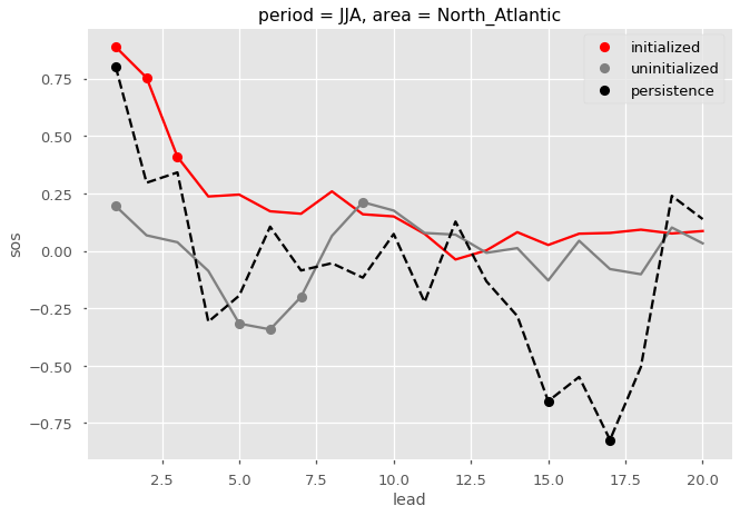
Here I plot the ACC for the initialized, uninitialized, and persistence forecasts for North Atlantic sea surface salinity in JJA. I add circles to the lines if the correlations are statistically significant for  .
.
[26]:
# ACC for initialized ensemble
acc = pm.compute_metric('acc')
acc.sos.plot(color='red')
acc.where(pm.compute_metric('p_pval') <= 0.05).sos.plot(marker='o', linestyle='None', color='red', label='initialized')

# ACC for 'uninitialized' ensemble
acc = pm.compute_uninitialized('acc')
acc.sos.plot(color='gray')
acc.where(pm.compute_uninitialized('p_pval') <= 0.05).sos.plot(marker='o', linestyle='None', color='gray', label='uninitialized')

# ACC for persistence forecast
acc = pm.compute_persistence('acc')
acc.sos.plot(color='k', linestyle='--')
acc.where(pm.compute_persistence('p_pval') <= 0.05).sos.plot(marker='o', linestyle='None', color='k', label='persistence')

plt.legend()
[26]:
<matplotlib.legend.Legend at 0x7fce7a441828>